Python
Algorithms
Mastering Basic Algorithms in the
Python Language
Magnus Lie Hetland
Learn to implement classic algorithms and design
new problem-solving algorithms using Python
•Transformnewproblemstowell-knownalgorithmicproblemswithefficient
•AnalyzealgorithmsandPythonprogramsbothusingmathematicaltoolsand
•Provecorrectness,optimality,orboundsonapproximationerrorforPython
•Understandseveralclassicalalgorithmsanddatastructuresindepth,andlearn
Python Algorithms
Mastering Basic Algorithms in the
Python Language
■ ■ ■
Python Algorithms: Mastering Basic Algorithms in the Python Language
Copyright © 2010 by Magnus Lie Hetland
All rights reserved. No part of this work may be reproduced or transmitted in any form or by any means, electronic or mechanical, including photocopying, recording, or by any information storage or retrieval system, without the prior written permission of the copyright owner and the publisher.
ISBN-13 (pbk): 978-1-4302-3237-7 ISBN-13 (electronic): 978-1-4302-3238-4
Printed and bound in the United States of America 9 8 7 6 5 4 3 2 1
Trademarked names, logos, and images may appear in this book. Rather than use a trademark symbol with every occurrence of a trademarked name, logo, or image we use the names, logos, and images only in an editorial fashion and to the benefit of the trademark owner, with no intention of infringement of the trademark.
The use in this publication of trade names, trademarks, service marks, and similar terms, even if they are not identified as such, is not to be taken as an expression of opinion as to whether or not they are subject to proprietary rights.
President and Publisher: Paul Manning Lead Editor: Frank Pohlmann
Development Editor: Douglas Pundick Technical Reviewer: Alex Martelli
Editorial Board: Steve Anglin, Mark Beckner, Ewan Buckingham, Gary Cornell, Jonathan Gennick, Jonathan Hassell, Michelle Lowman, Matthew Moodie, Duncan Parkes, Jeffrey Pepper, Frank Pohlmann, Douglas Pundick, Ben Renow-Clarke, Dominic Shakeshaft, Matt Wade, Tom Welsh Coordinating Editor: Adam Heath
Compositor: Mary Sudul Indexer: Brenda Miller Artist: April Milne
Cover Designer: Anna Ishchenko Photo Credit: Kai T. Dragland
Distributed to the book trade worldwide by Springer Science+Business Media, LLC., 233 Spring Street, 6th Floor, New York, NY 10013. Phone 1-800-SPRINGER, fax (201) 348-4505, e-mail
orders-ny@springer-sbm.com, or visit www.springeronline.com.
For information on translations, please e-mail rights@apress.com, or visit www.apress.com.
Apress and friends of ED books may be purchased in bulk for academic, corporate, or promotional use. eBook versions and licenses are also available for most titles. For more information, reference our Special Bulk Sales–eBook Licensing web page at www.apress.com/info/bulksales.
The information in this book is distributed on an “as is” basis, without warranty. Although every precaution has been taken in the preparation of this work, neither the author(s) nor Apress shall have any liability to any person or entity with respect to any loss or damage caused or alleged to be caused directly or indirectly by the information contained in this work.
For my students.
Contents at a Glance
Contents...vi
About the Author ...xiii
About the Technical Reviewer ... xiv
Acknowledgments ... xv
Preface ... xvi
■
Chapter 1: Introduction ...1
■
Chapter 2: The Basics ...9
■
Chapter 3: Counting 101 ...45
■
Chapter 4: Induction and Recursion … and Reduction...71
■
Chapter 5: Traversal: The Skeleton Key of Algorithmics ...101
■
Chapter 6: Divide, Combine, and Conquer...125
■
Chapter 7: Greed Is Good? Prove It!...151
■
Chapter 8: Tangled Dependencies and Memoization ...175
■
Chapter 9: From A to B with Edsger and Friends...199
■
Chapter 10: Matchings, Cuts, and Flows ...221
■
Chapter 11: Hard Problems and (Limited) Sloppiness ...241
■
Appendix A: Pedal to the Metal: Accelerating Python ...271
■
Appendix B: List of Problems and Algorithms ...275
■
Appendix C: Graph Terminology...285
■
Appendix D: Hints for Exercises...291
■ CONTENTS
Contents
Contents at a Glance...v
About the Author ...xiii
About the Technical Reviewer ... xiv
Acknowledgments ... xv
Preface ... xvi
■
Chapter 1: Introduction ...1
What’s All This, Then? ...2
Why Are You Here? ...3
Some Prerequisites ...4
What’s in This Book ...5
Summary ...6
If You’re Curious … ...6
Exercises ...7
References...7
■
Chapter 2: The Basics ...9
Some Core Ideas in Computing ...9
Asymptotic Notation ...10
It’s Greek to Me! ...12
Rules of the Road ...14
Taking the Asymptotics for a Spin...16
Three Important Cases ...19
Implementing Graphs and Trees...23
Adjacency Lists and the Like ...25
Adjacency Matrices ...29
Implementing Trees...32
A Multitude of Representations ...35
Beware of Black Boxes...36
Hidden Squares ...37
The Trouble with Floats ...38
Summary ...40
If You’re Curious … ...41
Exercises ...42
References...43
■
Chapter 3: Counting 101 ...45
The Skinny on Sums ...45
More Greek ...46
Working with Sums ...46
A Tale of Two Tournaments ...47
Shaking Hands...47
The Hare and the Tortoise ...49
Subsets, Permutations, and Combinations...53
Recursion and Recurrences...56
Doing It by Hand ...57
A Few Important Examples...58
Guessing and Checking ...62
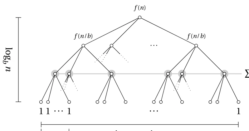
The Master Theorem: A Cookie-Cutter Solution ...64
So What Was All
That
About? ...67
Summary ...68
If You’re Curious … ...69
■ CONTENTS
References...70
■
Chapter 4: Induction and Recursion … and Reduction...71
Oh, That’s Easy! ...72
One, Two, Many ...74
Mirror, Mirror ...76
Designing with Induction (and Recursion) ...81
Finding a Maximum Permutation ...81
The Celebrity Problem ...85
Topological Sorting...87
Stronger Assumptions ...91
Invariants and Correctness...92
Relaxation and Gradual Improvement...93
Reduction + Contraposition = Hardness Proof ...94
Problem Solving Advice ...95
Summary ...96
If You’re Curious … ...97
Exercises ...97
References...99
■
Chapter 5: Traversal: The Skeleton Key of Algorithmics ...101
A Walk in the Park ...107
No Cycles Allowed ...108
How to Stop Walking in Circles ...109
Go Deep! ...110
Depth-First Timestamps and Topological Sorting (Again) ...112
Infinite Mazes and Shortest (Unweighted) Paths...114
Strongly Connected Components ...118
If You’re Curious … ...122
Exercises ...122
References...123
■
Chapter 6: Divide, Combine, and Conquer...125
Tree-Shaped Problems: All About the Balance...125
The Canonical D&C Algorithm...128
Searching by Halves ...129
Traversing Search Trees … with Pruning ...130
Selection...133
Sorting by Halves...135
How Fast Can We Sort? ...137
Three More Examples ...138
Closest Pair...138
Convex Hull...140
Greatest Slice ...142
Tree Balance … and Balancing...143
Summary ...148
If You’re Curious … ...149
Exercises ...149
References...150
■
Chapter 7: Greed Is Good? Prove It!...151
Staying Safe, Step by Step ...151
The Knapsack Problem ...155
Fractional Knapsack ...155
Integer Knapsack...156
Huffman’s Algorithm...156
The Algorithm ...158
■ CONTENTS
Going the Rest of the Way ...160
Optimal Merging ...160
Minimum spanning trees. ...161
The Shortest Edge ...162
What About the Rest? ...163
Kruskal’s Algorithm ...164
Prim’s Algorithm...166
Greed Works. But When?. ...168
Keeping Up with the Best ...168
No Worse Than Perfect...169
Staying Safe ...170
Summary . ...172
If You’re Curious … . ...172
Exercises ...173
References...174
■
Chapter 8: Tangled Dependencies and Memoization ...175
Don’t Repeat Yourself . ...176
Shortest Paths in Directed Acyclic Graphs . ...182
Longest Increasing Subsequence. ...184
Sequence Comparison. ...187
The Knapsack Strikes Back . ...190
Binary Sequence Partitioning . ...193
Summary . ...196
If You’re Curious … . ...196
Exercises . ...197
■
Chapter 9: From A to B with Edsger and Friends...199
Propagating Knowledge...200
Relaxing like Crazy ...201
Finding the Hidden DAG...204
All Against All...206
Far-Fetched Subproblems ...208
Meeting in the Middle...211
Knowing Where You’re Going ...213
Summary ...217
If You’re Curious … ...218
Exercises ...218
References...219
■
Chapter 10: Matchings, Cuts, and Flows ...221
Bipartite Matching ...222
Disjoint Paths...225
Maximum Flow ...227
Minimum Cut ...231
Cheapest Flow and the Assignment Problem ...232
Some Applications ...234
Summary ...237
If You’re Curious … ...237
Exercises ...238
References...239
■
Chapter 11: Hard Problems and (Limited) Sloppiness ...241
Reduction Redux...241
Not in Kansas Anymore?...244
■ CONTENTS
But Where Do You Start? And Where Do You Go from There?...249
A Ménagerie of Monsters...254
Return of the Knapsack ...254
Cliques and Colorings ...256
Paths and Circuits ...258
When the Going Gets Tough, the Smart Get Sloppy...261
Desperately Seeking Solutions ...263
And the Moral of the Story Is … ...265
Summary ...267
If You’re Curious … ...267
Exercises ...267
References...269
■
Appendix A: Pedal to the Metal: Accelerating Python ...271
■
Appendix B: List of Problems and Algorithms ...275
■
Appendix C: Graph Terminology...285
■
Appendix D: Hints for Exercises...291
About the Author
■ CONTENTS
About the Technical Reviewer
Acknowledgments
■ INTRODUCTION
Preface
■ ■ ■
Introduction
1. Write down the problem. 2. Think real hard.
3. Write down the solution.
“The Feynman Algorithm” as described by Murray Gell-Mann
Consider the following problem. You are to visit all the cities, towns, and villages of, say, Sweden and then return to your starting point. This might take a while (there are 24 978 locations to visit, after all), so you want to minimize your route. You plan on visiting each location exactly once, following the shortest route possible. As a programmer, you certainly don’t want to plot the route by hand. Rather, you try to write some code that will plan your trip for you. For some reason, however, you can’t seem to get it right. A straightforward program works well for a smaller number of towns and cities but seems to run forever on the actual problem, and improving the program turns out to be surprisingly hard. How come?
Actually, in 2004, a team of five researchers1 found such a tour of Sweden, after a number of other research teams had tried and failed. The five-man team used cutting-edge software with lots of clever optimizations and tricks of the trade, running on a cluster of 96 Xeon 2.6 GHz workstations. Their software ran from March 2003 until May 2004, before it finally printed out the optimal solution. Taking various interruptions into account, the team estimated that the total CPU time spent was about 85 years!
Consider a similar problem: You want to get from Kashgar, in the westernmost regions of China, to Ningbo, on the east coast, following the shortest route possible. Now, China has 3 583 715 km of roadways and 77 834 km of railways, with millions of intersections to consider and a virtually unfathomable number of possible routes to follow. It might seem that this problem is related to the previous one, yet this shortest path problem is one solved routinely, with no appreciable delay, by GPS software and online map services. If you give those two cities to your favorite map service, you should get the shortest route in mere moments. What’s going on here?
You will learn more about both of these problems later in the book; the first one is called the traveling salesman (or salesrep) problem and is covered in Chapter 11, while so-called shortest path problems are primarily dealt with in Chapter 9. I also hope you will gain a rather deep insight into why one problem seems like such a hard nut to crack while the other admits several well-known, efficient solutions. More importantly, you will learn something about how to deal with algorithmic and
computational problems in general, either solving them efficiently, using one of the several techniques and algorithms you encounter in this book, or showing that they are too hard and that approximate solutions may be all you can hope for. This chapter briefly describes what the book is about—what you
1
CHAPTER 1 ■ INTRODUCTION
can expect and what is expected of you. It also outlines the specific contents of the various chapters to come in case you want to skip around.
What’s All This, Then?
This is a book about algorithmic problem solving for Python programmers. Just like books on, say, object-oriented patterns, the problems it deals with are of a general nature—as are the solutions. Your task as an algorist will, in many cases, be more than simply to implement or execute an existing algorithm, as you would, for example, in solving an algebra problem. Instead, you are expected to come up with new algorithms—new general solutions to hitherto unseen, general problems. In this book, you are going to learn principles for constructing such solutions.
This may not be your typical algorithm book, though. Most of the authoritative books on the subject (such as the Knuth’s classics or the industry-standard textbook by Cormen et al.) have a heavy formal and theoretical slant, even though some of them (such as the one by Kleinberg and Tardos) lean more in the direction of readability. Instead of trying to replace any of these excellent books, I’d like to
supplement them. Building on my experience from teaching algorithms, I try to explain as clearly as possible how the algorithms work and what common principles underlie many of them. For a
programmer, these explanations are probably enough. Chances are you’ll be able to understand why the algorithms are correct and how to adapt them to new problems you may come to face. If, however, you need the full depth of the more formalistic and encyclopedic textbooks, I hope the foundation you get in this book will help you understand the theorems and proofs you encounter there.
There is another genre of algorithm books as well: the “(Data Structures and) Algorithms in blank” kind, where the blank is the author’s favorite programming language. There are quite a few of these (especially for blank = Java, it seems), but many of them focus on relatively basic data structures, to the detriment of the more meaty stuff. This is understandable if the book is designed to be used in a basic course on data structures, for example, but for a Python programmer, learning about singly and doubly linked lists may not be all that exciting (although you will hear a bit about those in the next chapter). And even though techniques such as hashing are highly important, you get hash tables for free in the form of Python dictionaries; there’s no need to implement them from scratch. Instead, I focus on more high-level algorithms. Many important concepts that are available as black-box implementations either in the Python language itself or in the standard library (such as sorting, searching, and hashing) are explained more briefly, in special “black box” sidebars throughout the text.
There is, of course, another factor that separates this book from those in the “Algorithms in Java/C/C++/C#” genre, namely, that the blank is Python. This places the book one step closer to the language-independent books (such as those by Knuth,2 Cormen et al., and Kleinberg and Tardos, for example), which often use pseudocode, the kind of fake programming language that is designed to be readable rather than executable. One of Python’s distinguishing features is its readability; it is, more or less, executable pseudocode. Even if you’ve never programmed in Python, you could probably decipher the meaning of most basic Python programs. The code in this book is designed to be readable exactly in this fashion—you need not be a Python expert to understand the examples (although you might need to look up some built-in functions and the like). And if you want to pretend the examples are actually pseudocode, feel free to do so. To sum up …
2
What the book is about:
• Algorithm analysis, with a focus on asymptotic running time
• Basic principles of algorithm design
• How to represent well-known data structures in Python
• How to implement well-known algorithms in Python
What the book covers only briefly or partially:
• Algorithms that are directly available in Python, either as part of the language or via the standard library
• Thorough and deep formalism (although the book has its share of proofs and proof-like explanations)
What the book isn’t about:3
• Numerical or number-theoretical algorithms (except for some floating-point hints in Chapter 2)
• Parallel algorithms and multicore programming
As you can see, “implementing things in Python” is just part of the picture. The design principles and theoretical foundations are included in the hope that they’ll help you design your own algorithms and data structures.
Why Are You Here?
When working with algorithms, you’re trying to solve problems efficiently. Your programs should be fast; the wait for a solution should be short. But what, exactly, do we mean by efficient, fast, and short? And why would one care about these things in a language such as Python, which isn’t exactly lightning fast to begin with? Why not rather switch to, say, C or Java?
First, Python is a lovely language, and you may not want to switch. Or maybe you have no choice in the matter. But second, and perhaps most importantly, algorists don’t primarily worry about constant differences in performance.4 If one program takes twice, or even ten times, as long as another to finish, it may still be fast enough, and the slower program (or language) may have other desirable properties, such as being more readable. Tweaking and optimizing can be costly in many ways and is not a task to be taken on lightly. What does matter, though, no matter the language, is how your program scales. If you double the size of your input, what happens? Will your program run for twice as long? Four times? More? Will the running time double even if you add just one measly bit to the input? These are the kind of differences that will easily trump language or hardware choice, if your problems get big enough. And in some cases “big enough” needn’t be all that big. Your main weapon in whittling down the growth of your running time is—you guessed it—a solid understanding of algorithm design.
Let’s try a little experiment. Fire up an interactive Python interpreter, and enter the following:
3
Of course, the book is also not about a lot of other things ….
4
CHAPTER 1 ■ INTRODUCTION
>>> count = 10**5 >>> nums = []
>>> for i in range(count): ... nums.append(i) ...
>>> nums.reverse()
Not the most useful piece of code, perhaps. It simply appends a bunch of numbers to an (initially) empty list and then reverses that list. In a more realistic situation, the numbers might come from some outside source (they could be incoming connections to a server, for example), and you want to add them to your list in reverse order, perhaps to prioritize the most recent ones. Now you get an idea: instead of reversing the list at the end, couldn’t you just insert the numbers at the beginning, as they appear? Here’s an attempt to streamline the code (continuing in the same interpreter window):
>>> nums = []
>>> for i in range(count): ... nums.insert(0, i)
Unless you’ve encountered this situation before, the new code might look promising, but try to run it. Chances are you’ll notice a distinct slowdown. On my computer, the second piece of code takes over 100 times as long as the first to finish. Not only is it slower, but it also scales worse with the problem size. Try, for example, to increase count from 10**5 to 10**6. As expected, this increases the running time for the first piece of code by a factor of about ten … but the second version is slowed by roughly two orders of magnitude, making it more than a thousand times slower than the first! As you can probably guess, the discrepancy between the two versions only increases as the problem gets bigger, making the choice between them ever more crucial.
■Note This is an example of linear vs. quadratic growth, a topic dealt with in detail in Chapter 3. The specific issue underlying the quadratic growth is explained in the discussion of vectors (or dynamic arrays) in the black box sidebar on list in Chapter 2.
Some Prerequisites
This book is intended for two groups of people: Python programmers, who want to beef up their algorithmics, and students taking algorithm courses, who want a supplement to their plain-vanilla algorithms textbook. Even if you belong to the latter group, I’m assuming you have a familiarity with programming in general and with Python in particular. If you don’t, perhaps my book Beginning Python (which covers Python versions up to 3.0) can help? The Python web site also has a lot of useful material, and Python is a really easy language to learn. There is some math in the pages ahead, but you don’t have to be a math prodigy to follow the text. We’ll be dealing with some simple sums and nifty concepts such as polynomials, exponentials, and logarithms, but I’ll explain it all as we go along.
reason, you’re still stuck with, say, the Python 1.5 series, most of the code should still work, with a tweak here and there.)
GETTING WHAT YOU NEED
In some operating systems, such as Mac OS X and several flavors of Linux, Python should already be installed. If it is not, most Linux distributions will let you install the software you need through some form of package manager. If you want or need to install Python manually, you can find all you need on the Python web site, http://python.org.
What’s in This Book
The book is structured as follows:Chapter 1: Introduction. You’ve already gotten through most of this. It gives an overview of the book.
Chapter 2: The Basics. This covers the basic concepts and terminology, as well as some fundamental math. Among other things, you learn how to be sloppier with your formulas than ever before, and still get the right results, with asymptotic notation.
Chapter 3: Counting 101. More math—but it’s really fun math, I promise! There’s some basic
combinatorics for analyzing the running time of algorithms, as well as a gentle introduction to recursion and recurrence relations.
Chapter 4: Induction and Recursion … and Reduction. The three terms in the title are crucial, and they are closely related. Here we work with induction and recursion, which are virtually mirror images of each other, both for designing new algorithms and for proving correctness. We also have a somewhat briefer look at the idea of reduction, which runs as a common thread through almost all algorithmic work.
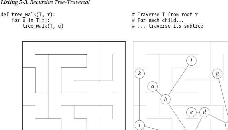
Chapter 5: Traversal: A Skeleton Key to Algorithmics. Traversal can be understood using the ideas of induction and recursion, but it is in many ways a more concrete and specific technique. Several of the algorithms in this book are simply augmented traversals, so mastering traversal will give you a real jump start.
Chapter 6: Divide, Combine, and Conquer. When problems can be decomposed into independent subproblems, you can recursively solve these subproblems and usually get efficient, correct algorithms as a result. This principle has several applications, not all of which are entirely obvious, and it is a mental tool well worth acquiring.
Chapter 7: Greed is Good? Prove It! Greedy algorithms are usually easy to construct. One can even formulate a general scheme that most, if not all, greedy algorithms follow, yielding a plug-and-play solution. Not only are they easy to construct, but they are usually very efficient. The problem is, it can be hard to show that they are correct (and often they aren’t). This chapter deals with some well-known examples and some more general methods for constructing correctness proofs.
CHAPTER 1 ■ INTRODUCTION
Chapter 9: From A to B with Edsger and Friends. Rather than the design methods of the previous three chapters, we now focus on a specific problem, with a host of applications: finding shortest paths in networks, or graphs. There are many variations of the problem, with corresponding (beautiful) algorithms.
Chapter 10: Matchings, Cuts, and Flows. How do you match, say, students with colleges so you
maximize total satisfaction? In an online community, how do you know whom to trust? And how do you find the total capacity of a road network? These, and several other problems, can be solved with a small class of closely related algorithms and are all variations of the maximum flow problem, which is covered in this chapter.
Chapter 11: Hard Problems and (Limited) Sloppiness. As alluded to in the beginning of the
introduction, there are problems we don’t know how to solve efficiently and that we have reasons to think won’t be solved for a long time—maybe never. In this chapter, you learn how to apply the trusty tool of reduction in a new way: not to solve problems but to show that they are hard. Also, we have a look at how a bit of (strictly limited) sloppiness in our optimality criteria can make problems a lot easier to solve.
Appendix A: Pedal to the Metal: Accelerating Python. The main focus of this book is asymptotic efficiency—making your programs scale well with problem size. However, in some cases, that may not be enough. This appendix gives you some pointers to tools that can make your Python programs go faster. Sometimes a lot (as in hundreds of times) faster.
Appendix B: List of Problems and Algorithms. This appendix gives you an overview of the algorithmic problems and algorithms discussed in the book, with some extra information to help you select the right algorithm for the problem at hand.
Appendix C: Graph Terminology and Notation. Graphs are a really useful structure, both in describing real-world systems and in demonstrating how various algorithms work. This chapter gives you a tour of the basic concepts and lingo, in case you haven’t dealt with graphs before.
Appendix D: Hints for Exercises. Just what the title says.
Summary
Programming isn’t just about software architecture and object-oriented design; it’s also about solving algorithmic problems, some of which are really hard. For the more run-of-the-mill problems (such as finding the shortest path from A to B), the algorithm you use or design can have a huge impact on the time your code takes to finish, and for the hard problems (such as finding the shortest route through A–Z), there may not even be an efficient algorithm, meaning that you need to accept approximate solutions.
This book will teach you several well-known algorithms, along with general principles that will help you create your own. Ideally, this will let you solve some of the more challenging problems out there, as well as create programs that scale gracefully with problem size. In the next chapter, we get started with the basic concepts of algorithmics, dealing with terms that will be used throughout the entire book.
If You’re Curious …
Exercises
As with the previous section, this is one you’ll encounter again and again. Hints for solving the exercises can be found at the back of the book. The exercises often tie in with the main text, covering points that aren’t explicitly discussed there but that may be of interest or that deserve some contemplation. If you want to really sharpen your algorithm design skills, you might also want to check out some of the myriad of sources of programming puzzles out there. There are, for example, lots of programming contests (a web search should turn up plenty), many of which post problems that you can play with. Many big software companies also have qualification tests based on problems such as these and publish some of them online.
Because the introduction doesn’t cover that much ground, I’ll just give you a couple of exercises here—a taste of what’s to come:
1-1. Consider the following statement: “As machines get faster and memory cheaper, algorithms become less important.” What do you think; is this true or false? Why?
1-2. Find a way of checking whether two strings are anagrams of each other (such as "debitcard" and "badcredit"). How well do you think your solution scales? Can you think of a naïve solution that will scale very poorly?
References
Applegate, D., Bixby, R., Chvátal, V., Cook, W., and Helsgaun, K. Optimal tour of Sweden. http://www.tsp.gatech.edu/sweden. Accessed September 12, 2010.
Cormen, T. H., Leiserson, C. E., Rivest, R. L., and Stein, C. (2009). Introduction to Algorithms, second edition. MIT Press.
Dasgupta, S., Papadimitriou, C., and Vazirani, U. (2006). Algorithms. McGraw-Hill.
Goodrich, M. T. and Tamassia, R. (2001). Algorithm Design: Foundations, Analysis, and Internet Examples. John Wiley & Sons, Ltd.
Hetland, M. L. (2008). Beginning Python: From Novice to Professional, second edition. Apress.
Kleinberg, J. and Tardos, E. (2005). Algorithm Design. Addison-Wesley Longman Publishing Co., Inc.
Knuth, D. E. (1968). Fundamental Algorithms, volume 1 of The Art of Computer Programming. Addison-Wesley.
———. (1969). Seminumerical Algorithms, volume 2 of The Art of Computer Programming. Addison-Wesley.
———. (1973). Sorting and Searching, volume 3 of The Art of Computer Programming. Addison-Wesley.
———. (2005a). Generating All Combinations and Partitions, volume 4, fascicle 3 of The Art of Computer Programming. Addison-Wesley.
———. (2005b). Generating All Tuples and Permutations, volume 4, fascicle 2 of The Art of Computer Programming. Addison-Wesley.
CHAPTER 1 ■ INTRODUCTION
———. (2008). Introduction to Combinatorial Algorithms and Boolean Functions, volume 4, fascicle 0 of The Art of Computer Programming. Addison-Wesley.
■ ■ ■
The Basics
Tracey: I didn’t know you were out there.
Zoe: Sort of the point. Stealth—you may have heard of it. Tracey: I don’t think they covered that in basic.
From “The Message,” episode 14 of Firefly
Before moving on to the mathematical techniques, algorithmic design principles, and classical algorithms that make up the bulk of this book, we need to go through some basic principles and techniques. When you start reading the following chapters, you should be clear on the meaning of phrases such as “directed, weighted graph without negative cycles” and “a running time of Θ(n lg n).” You should also have an idea of how to implement some fundamental structures in Python.
Luckily, these basic ideas aren’t at all hard to grasp. The main two topics of the chapter are asymptotic notation, which lets you focus on the essence of running times, and ways of representing trees and graphs in Python. There is also practical advice on timing your programs and avoiding some basic traps. First, though, let’s take a look at the abstract machines we algorists tend to use when describing the behavior of our algorithms.
Some Core Ideas in Computing
In the mid-1930s the English mathematician Alan Turing published a paper called “On computable numbers, with an application to the Entscheidungsproblem”1 and, in many ways, laid the groundwork for modern computer science. His abstract Turing machine has become a central concept in the theory of computation, in great part because it is intuitively easy to grasp. A Turing machine is a simple
(abstract) device that can read from, write to, and move along an infinitely long strip of paper. The actual behavior of the machines varies. Each is a so-called finite state machine: it has a finite set of states (some of which indicate that it has finished), and every symbol it reads potentially triggers reading and/or writing and switching to a different state. You can think of this machinery as a set of rules. (“If I am in state 4 and see an X, I move one step to the left, write a Y, and switch to state 9.”) Although these machines may seem simple, they can, surprisingly enough, be used to implement any form of computation anyone has been able to dream up so far, and most computer scientists believe they encapsulate the very essence of what we think of as computing.
1
CHAPTER 2 ■ THE BASICS
An algorithm is a procedure, consisting of a finite set of steps (possibly including loops and conditionals) that solves a given problem in finite time. A Turing machine is a formal description of exactly what problem an algorithm solves,2 and the formalism is often used when discussing which problems can be solved (either at all or in reasonable time, as discussed later in this chapter and in Chapter 11). For more fine-grained analysis of algorithmic efficiency, however, Turing machines are not usually the first choice. Instead of scrolling along a paper tape, we use a big chunk of memory that can be accessed directly. The resulting machine is commonly known as the random-access machine.
While the formalities of the random-access machine can get a bit complicated, we just need to know something about the limits of its capabilities so we don’t cheat in our algorithm analyses. The machine is an abstract, simplified version of a standard, single-processor computer, with the following properties:
• We don’t have access to any form of concurrent execution; the machine simply executes one instruction after the other.
• Standard, basic operations (such as arithmetic, comparisons, and memory access) all take constant (although possibly different) amounts of time. There are no more complicated basic operations (such as sorting).
• One computer word (the size of a value that we can work with in constant time) is not unlimited but is big enough to address all the memory locations used to represent our problem, plus an extra percentage for our variables.
In some cases, we may need to be more specific, but this machine sketch should do for the moment. We now have a bit of an intuition for what algorithms are, as well as the (abstract) hardware we’ll be running them on. The last piece of the puzzle is the notion of a problem. For our purposes, a
problem is a relation between input and output. This is, in fact, much more precise than it might sound: a relation (in the mathematical sense) is a set of pairs—in our case, which outputs are acceptable for which inputs—and by specifying this relation, we’ve got our problem nailed down. For example, the problem of sorting may be specified as a relation between two sets, A and B, each consisting of sequences.3 Without describing how to perform the sorting (that would be the algorithm), we can specify which output sequences (elements of B) that would be acceptable, given an input sequence (an element of A). We would require that the result sequence consisted of the same elements as the input sequence and that the elements of the result sequence were in increasing order (each bigger than or equal to the previous). The elements of A here (that is, the inputs) are called problem instances; the relation itself is the actual problem.
To get our machine to work with a problem, we need to encode the input as zeros and ones. We won’t worry too much about the details here, but the idea is important, because the notion of running time complexity (as described in the next section) is based on knowing how big a problem instance is, and that size is simply the amount of memory needed to encode it. (As you’ll see, the exact nature of this encoding usually won’t matter.)
Asymptotic Notation
Remember the append versus insert example in Chapter 1? Somehow, adding items to the end of a list scaled better with the list size than inserting them at the front (see the nearby black box sidebar on list
for an explanation). These built-in operations are both written in C, but assume for a minute that you reimplement list.append in pure Python; let’s say (arbitrarily) that the new version is 50 times slower
2
There are also Turing machines that don’t solve any problems—machines that simply never stop. These still represent what we might call programs, but we usually don’t call them algorithms.
3
than the original. Let’s also say that you run your slow, pure-Python append-based version on a really slow machine, while the fast, optimized, insert-based version is run on a computer that is 1000 times faster. Now the speed advantage of the insert version is a factor of 50 000. You compare the two implementations by inserting 100 000 numbers. What do you think happens?
Intuitively, it might seem obvious that the speedy solution should win, but its “speediness” is just a constant factor, and its running time grows faster than the “slower” one. For the example at hand, the Python-coded version running on the slower machine will, actually, finish in half the time of the other one. Let’s increase the problem size a bit, to 10 million numbers, for example. Now the Python version on the slow machine will be 2000 times faster than the C version on the fast machine. That’s like the difference between running for about a minute and running almost a day and a half!
This distinction between constant factors (related to such things as general programming language performance and hardware speed, for example) and the growth of the running time, as problem sizes increase, is of vital importance in the study of algorithms. Our focus is on the big picture—the implementation-independent properties of a given way of solving a problem. We want to get rid of distracting details and get down to the core differences, but in order to do so, we need some formalism.
BLACK BOX: LIST
Python lists aren’t really lists in the traditional (computer science) sense of the word, and that explains the puzzle of why append is so much more efficient than insert. A classical list—a so-called linked list—is implemented as a series of nodes, each (except for the last) keeping a reference to the next. A simple implementation might look something like this:
class Node:
def __init__(self, value, next=None): self.value = value
self.next = next
You construct a list by specifying all the nodes:
>>> L = Node("a", Node("b", Node("c", Node("d")))) >>> L.next.next.value
'c'
This is a so-called singly linked list; each node in a doubly linked list would also keep a reference to the previous node.
CHAPTER 2 ■ THE BASICS
The difference we’ve been bumping up against, though, has to do with insertion. In a linked list, once you know where you want to insert something, insertion is cheap; it takes (roughly) the same amount of time, no matter how many elements the list contains. Not so with arrays: an insertion would have to move all elements that are to the right of the insertion point, possibly even moving all the elements to a larger array, if needed. A specific solution for appending is to use what’s often called a dynamic array, or vector.4
The idea is to allocate an array that is too big and then to reallocate it (in linear time) whenever it overflows. It might seem that this makes the append just as bad as the insert. In both cases, we risk having to move a large number of elements. The main difference is that it happens less often with the append. In fact, if we can ensure that we always move to an array that is bigger than the last by a fixed percentage (say 20 percent or even 100 percent), the average cost (or, more correctly, the amortized cost, averaged over many appends) is negligible (constant).
It’s Greek to Me!
Asymptotic notation has been in use (with some variations) since the late 19th century and is an essential tool in analyzing algorithms and data structures. The core idea is to represent the resource we’re analyzing (usually time but sometimes also memory) as a function, with the input size as its parameter. For example, we could have a program with a running time of T(n) = 2.4n + 7.
An important question arises immediately: what are the units here? It might seem trivial whether we measure the running time in seconds or milliseconds or whether we use bits or megabytes to represent problem size. The somewhat surprising answer, though, is that not only is it trivial, but it actually will not affect our results at all. We could measure time in Jovian years and problem size in kg (presumably the mass of the storage medium used), and it will not matter. This is because our original intention of ignoring implementation details carries over to these factors as well: the asymptotic notation ignores them all! (We do normally assume that the problem size is a positive integer, though.)
What we often end up doing is letting the running time be the number of times a certain basic operation is performed, while problem size is either the number of items handled (such as the number of integers to be sorted, for example) or, in some cases, the number of bits needed to encode the problem instance in some reasonable encoding.
Forgetting. Of course, the assert doesn’t work. (http://xkcd.com/379)
4
■Note Exactly how you encode your problems and solutions as bit patterns usually has little effect on the asymptotic running time, as long as you are reasonable. For example, avoid representing your numbers in the unary number system (1=1, 2=11, 3=111…).
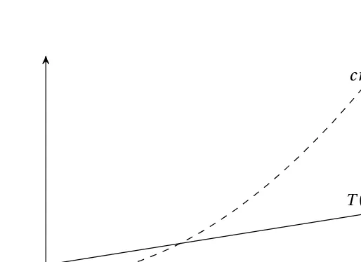
The asymptotic notation consists of a bunch of operators, written as Greek letters. The most important ones (and the only ones we’ll be using) are O (originally an omicron but now usually called “Big Oh”), Ω (omega), and Θ (theta). The definition for the O operator can be used as a foundation for the other two. The expression O(g), for some function g(n), represents a set of functions, and a function f(n) is in this set if it satisfies the following condition: there exists a natural number n0 and a positive constant c such that
f(n) ≤ cg(n)
for all n ≥ n0. In other words, if we’re allowed to tweak the constant c (for example, by running the algorithms on machines of different speeds), the function g will eventually (that is, at n0) grow bigger than f. See Figure 2-1 for an example.
This is a fairly straightforward and understandable definition, although it may seem a bit foreign at first. Basically, O(g) is the set of functions that do not grow faster than g. For example, the function n2 is in the set O(n2), or, in set notation, n2
∈ O(n2). We often simply say that n2 is O(n2).
The fact that n2 does not grow faster than itself is not particularly interesting. More useful, perhaps, is the fact that neither 2.4n2 + 7 nor the linear function n does. That is, we have both
2.4n2 + 7 ∈ O(n2)
and
n ∈ O(n2).
cn
2T
(
n
)
n
0CHAPTER 2 ■ THE BASICS
The first example shows us that we are now able to represent a function without all its bells and whistles; we can drop the 2.4 and the 7 and simply express the function as O(n2), which gives us just the information we need. The second shows us that O can be used to express loose limits as well: any function that is better (that is, doesn’t grow faster) than g can be found in O(g).
How does this relate to our original example? Well, the thing is, even though we can’t be sure of the details (after all, they depend on both the Python version and the hardware you’re using), we can describe the operations asymptotically: the running time of appending n numbers to a Python list is O(n), while inserting n numbers at its beginning is O(n2).
The other two, Ω and Θ, are just variations of O. Ω is its complete opposite: a function f is in Ω(g) if it satisfies the following condition: there exists a natural number n0 and a positive constant c such that
f(n) ≥ cg(n)
for all n ≥ n0. So, where O forms a so-called asymptotic upper bound, Ω forms an asymptotic lower bound.
■Note Our first two asymptotic operators, O and Ω, are each others’ inverses: if f is O(g), then g is Ω(f ). Exercise 1–3 asks you to show this.
The sets formed by Θ are simply intersections of the other two, that is, Θ(g) = O(g) ∩Ω(g). In other words, a function f is in Θ(g) if it satisfies the following condition: there exists a natural number n0 and two positive constants c1 and c2 such that
c1g(n) ≤f(n) ≤c2g(n)
for all n≥n0. This means that f and g have the same asymptotic growth. For example, 3n2 + 2 is Θ(n2), but we could just as well write that n2 is Θ(3n2 + 2). By supplying an upper bound and a lower bound at the same time, the Θ operator is the most informative of the three, and I will use it when possible.
Rules of the Road
While the definitions of the asymptotic operators can be a bit tough to use directly, they actually lead to some of the simplest math ever. You can drop all multiplicative and additive constants, as well as all other “small parts” of your function, which simplifies things a lot.
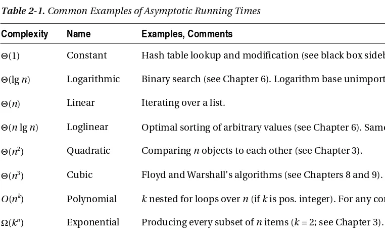
As a first step in juggling these asymptotic expressions, let’s take a look at some typical asymptotic classes, or orders. Table 2-1 lists some of these, along with their names and some typical algorithms with these asymptotic running times, also sometimes called running-time complexities. (If your math is a little rusty, you could take a look at the sidebar named “A Quick Math Refresher” later in the chapter.) An important feature of this table is that the complexities have been ordered so that each row dominates the previous one: if f is found lower in the table than g, then f is O(g).5
5
■Note Actually, the relationship is even stricter: f is o(g), where the “Little Oh” is a stricter version if “Big Oh.” Intuitively, instead of “doesn’t grow faster than,” it means “grows slower than.” Formally, it states that f(n) /g(n) converges to zero as n grows to infinity. You don’t really need to worry about this, though.
Any polynomial (that is, with any power k > 0, even a fractional one) dominates any logarithm (that is, with any base), and any exponential (with any base k > 1) dominates any polynomial (see Exercises 2-5 and 2-6). Actually, all logarithms are asymptotically equivalent—they differ only by constant factors (see Exercise 2-4). Polynomials and exponentials, however, have different asymptotic growth depending on their exponents or bases, respectively. So, n5 grows faster than n4, and 5n grows faster than 4n.
The table primarily uses Θ notation, but the terms polynomial and exponential are a bit special, because of the role they play in separating tractable (“solvable”) problems from intractable
(“unsolvable”) ones, as discussed in Chapter 11. Basically, an algorithm with a polynomial running time is considered feasible, while an exponential one is generally useless. Although this isn’t entirely true in practice, (Θ(n100) is no more practically useful than Θ(2n)), it is, in many cases, a useful distinction.6 Because of this division, any running time in O(nk), for any k > 0, is called polynomial, even though the limit may not be tight. For example, even though binary search (explained in the black box sidebar on
bisect in Chapter 6) has a running time of Θ(lg n), it is still said to be a polynomial-time (or just polynomial) algorithm. Conversely, any running time in Ω(kn)—even one that is, say, Θ(n!)—is said to be exponential.
Table 2-1. Common Examples of Asymptotic Running Times
Complexity Name Examples, Comments
Θ(1) Constant Hash table lookup and modification (see black box sidebar on dict).
Θ(lg n) Logarithmic Binary search (see Chapter 6). Logarithm base unimportant.
Θ(n) Linear Iterating over a list.
Θ(n lg n) Loglinear Optimal sorting of arbitrary values (see Chapter 6). Same as Θ(lg n!).
Θ(n2) Quadratic Comparing n objects to each other (see Chapter 3).
Θ(n3) Cubic Floyd and Warshall’s algorithms (see Chapters 8 and 9).
O(nk) Polynomial k nested for loops over n (if k is pos. integer). For any constant k > 0.
Ω(kn) Exponential Producing every subset of n items (k =2; see Chapter 3). Any k > 1.
Θ(n!) Factorial Producing every ordering of n values.
6
CHAPTER 2 ■ THE BASICS
Now that we have an overview of some important orders of growth, we can formulate two simple rules:
• In a sum, only the dominating summand matters. For example, Θ(n2 + n3 + 42) = Θ(n3).
• In a product, constant factors don’t matter. For example, Θ(4.2n lg n) = Θ(n lg n).
In general, we try to keep the asymptotic expressions as simple as possible, eliminating as many unnecessary parts as we can. For O and Ω, there is a third principle we usually follow:
• Keep your upper or lower limits tight.
In other words, we try to make the upper limits low and the lower limits high. For example, although n2 might technically be O(n3), we usually prefer the tighter limit, O(n2). In most cases, though, the best thing is to simply use Θ.
A practice that can make asymptotic expressions even more useful is that of using them instead of actual values, in arithmetic expressions. Although this is technically incorrect (each asymptotic expression yields a set of functions, after all), it is quite common. For example, Θ(n2) + Θ(n3) simply means f + g, for some (unknown) functions f and g, where f is Θ(n2) and g is Θ(n3). Even though we cannot find the exact sum f + g, because we don’t know the exact functions, we can find the asymptotic expression to cover it, as illustrated by the following two “bonus rules:”
• Θ(f) + Θ(g) = Θ(f + g)
• Θ(f) · Θ(g) = Θ(f · g)
Exercise 2-8 asks you to show that these are correct.
Taking the Asymptotics for a Spin
Let’s take a look at some very simple programs and see whether we can determine their asymptotic running times. To begin with, let’s consider programs where the (asymptotic) running time varies only with the problem size, not the specifics of the instance in question. (The next section deals with what happens if the actual contents of the instances matter to the running time.) This means, for example, that if statements are rather irrelevant for now. What’s important is loops, in addition to straightforward code blocks. Function calls don’t really complicate things; they just calculate the complexity for the call and insert it at the right place.
■Note There is one situation where function calls can trip us up: when the function is recursive. This case is dealt with in Chapters 3 and 4.
The loop-free case is simple: we are executing one statement before another, so their complexities are added. Let’s say, for example, that we know that for a list of size n, a call to append is Θ(1), while a call to insert at position 0 is Θ(n). Consider the following little two-line program fragment, where nums is a list of size n:
We know that the line first takes constant time. At the time we get to the second line, the list size has changed and is now n + 1. This means that the complexity of the second line is Θ(n + 1), which is the same as Θ(n). Thus, the total running time is the sum of the two complexities, Θ(1) + Θ(n) = Θ(n).
Now, let’s consider some simple loops. Here’s a plain for loop over a sequence with n elements (numbers, say):7
s = 0
for x in seq: s += x
This is a straightforward implementation of what the sum function does: it iterates over seq and adds the elements to the starting value in s. This performs a single constant-time operation (s+=x) for each of the n elements of seq, which means that its running time is linear, or Θ(n). Note that the constant-time initialization (s=0) is dominated by the loop here.
The same logic applies to the “camouflaged” loops we find in list (or set or dict) comprehensions and generator expressions, for example. The following list comprehension also has a linear running-time complexity:
squares = [x**2 for x in seq]
Several built-in functions and methods also have “hidden” loops in them. This generally applies to any function or method that deals with every element of a container, such as sum or map, for example.
Things get a little bit (but not a lot) trickier when we start nesting loops. Let’s say we want to sum up all possible products of the elements in seq, for example:
s = 0
for x in seq: for y in seq: s += x*y
One thing worth noting about this implementation is that each product will be added twice (if 42
and 333 are both in seq, for example, we’ll add both 42*333 and 333*42). That doesn’t really affect the running time (it’s just a constant factor).
What’s the running time now? The basic rule is easy: the complexities of code blocks executed one after the other are just added. The complexities of nested loops are multiplied. The reasoning is simple: for each round of the outer loop, the inner one is executed in full. In this case, that means “linear times linear,” which is quadratic. In other words, the running time is Θ(n·n) = Θ(n2). Actually, this
multiplication rule means that for further levels of nesting, we will just increment the power (that is, the exponent). Three nested linear loops give us Θ(n3), four give us Θ(n4), and so forth.
The sequential and nested cases can be mixed, of course. Consider the following slight extension:
s = 0
for x in seq: for y in seq: s += x*y for z in seq: for w in seq: s += x-w
7
CHAPTER 2 ■ THE BASICS
It may not be entirely clear what we’re computing here (I certainly have no idea), but we should still be able to find the running time, using our rules. The z-loop is run for a linear number of iterations, and it contains a linear loop, so the total complexity there is quadratic, or Θ(n2). The y-loop is clearly Θ(n). This means that the code block inside the x-loop is Θ(n + n2). This entire block is executed for each round of the x-loop, which is run n times. We use our multiplication rule and get Θ(n(n + n2)) = Θ(n2 + n3) = Θ(n3), that is, cubic. We could arrive at this conclusion even more easily by noting that the y-loop is dominated by the z-loop and can be ignored, giving the inner block a quadratic running time. “Quadratic times linear” gives us cubic.
The loops need not all be repeated Θ(n) times, of course. Let’s say we have two sequences, seq1 and
seq2, where seq1 contains n elements and seq2 contains m elements. The following code will then have a running time of Θ(nm):
s = 0
for x in seq1: for y in seq2: s += x*y
In fact, the inner loop need not even be executed the same number of times for each iteration of the outer loop. This is where things can get a bit fiddly. Instead of just multiplying two iteration counts (such as n and m in the previous example), we now have to sum the iteration counts of the inner loop. What that means should be clear in the following example:
seq1 = [[0, 1], [2], [3, 4, 5]] s = 0
for seq2 in seq1: for x in seq2: s += x
The statement s+=x is now performed 2 + 1 + 3 = 6 times. The length of seq2 gives us the running time of the inner loop, but because it varies, we cannot simply multiply it by the iteration count of the outer loop. A more realistic example is the following, which revisits our original example—multiplying every combination of elements from a sequence:
s = 0 n = len(seq)
for i in range(n-1): for j in range(i+1, n): s += seq[i] * seq[j]
To avoid multiplying objects with themselves or adding the same product twice, the outer loop now avoids the last item, and the inner loop iterates over the items only after the one currently considered by the outer one. This is actually a lot less confusing than it might seem, but finding the complexity here requires a little bit more care. This is one of the important cases of counting that is covered in the next chapter.8
8
Spoiler: The complexity of this example is still Θ(n2
Three Important Cases
Until now, we have assumed that the running time is completely deterministic and dependent only on input size, not on the actual contents of the input. That is not particularly realistic, however. For example, if you were to construct a sorting algorithm, you might start like this:
def sort_w_check(seq): n = len(seq)
for i in range(n-1): if seq[i] > seq[i+1]: break
else: return ...
A check is performed before getting into the actual sorting: if the sequence is already sorted, the function simply returns.
■Note The optional else clause on a loop in Python is executed if the loop has not been ended prematurely by a
break statement.
This means that no matter how inefficient our main sorting is, the running time will always be linear if the sequence is already sorted. No sorting algorithm can achieve linear running time in general, meaning that this “best-case scenario” is an anomaly—and all of a sudden, we can’t reliably predict the running time anymore. The solution to this quandary is to be more specific. Instead of talking about a problem in general, we can specify the input more narrowly, and we often talk about one of three important cases:
• The best case. This is the running time you get when the input is optimally suited to your algorithm. For example, if the input sequence to sort_w_check were sorted, we would get the best-case running time (which would be linear).
• The worst case. This is usually the most useful case—the worst possible running time. This is useful because we normally want to be able to give some guarantees about the efficiency of our algorithm, and this is the best guarantee we can give in general.
• The average case. This is a tricky one, and I’ll avoid it most of the time, but in some cases it can be useful. Simply put, it’s the expected value of the running time, for random input (with a given probability distribution).
In many of the algorithms we’ll be working with, these three cases have the same complexity. When they don’t, we’ll often be working with the worst case. Unless this is stated explicitly, however, no assumptions can be made about which case is being studied. In fact, we may not be restricting ourselves to a single kind of input at all. What if, for example, we wanted to describe the running time of
sort_w_checkin general? This is still possible, but we can’t be quite as precise.
CHAPTER 2 ■ THE BASICS
general, however—for any kind of input—we cannot use the Θ notation at all. There is no single function describing the running time; different types of inputs have different running time functions, and these have different asymptotic complexity, meaning we can’t sum them up in a single Θ expression.
The solution? Instead of the “twin bounds” of Θ, we only supply an upper or lower limit, using O or Ω. We can, for example, say that sort_w_check has a running time of O(n lg n). This covers both the best and worst cases. Similarly, we could say it has a running time of Ω(n). Note that these limits are as tight as we can make them.
■Note It is perfectly acceptable to use either of our asymptotic operators to describe either of the three cases discussed here. We could very well say that the worst-case running time of sort_w_check is Ω(n lg n), for example, or that the best case is O(n).
Empirical Evaluation of Algorithms
The main focus of this book is algorithm design (and its close relative, algorithm analysis). There is, however, another important discipline of algorithmics that can be of vital importance when building real-world systems, and that is algorithm engineering, the art of efficiently implementing algorithms. In a way, algorithm design can be seen as a way of achieving low asymptotic running time (by designing efficient algorithms), while algorithm engineering is focused on reducing the hidden constants in that asymptotic complexity.
Although I may offer some tips on algorithm engineering in Python here and there, it can be hard to predict exactly which tweaks and hacks will give you the best performance for the specific problems you’re working on—or, indeed, for your hardware or version of Python. (These are exactly the kind of quirks asymptotics are designed to avoid.) And in some cases, such tweaks and hacks may not be needed at all, because your program may be fast enough as it is. The most useful thing you can do in many cases is simply to try and see. If you have a tweak you think will improve your program, try it! Implement the tweak, and run some experiments. Is there an improvement? And if the tweak makes your code less readable and the improvement is small, is it really worth it?
■Note This section is about evaluating your programs, not on the engineering itself. For some hints on speeding up Python programs, see Appendix A.
While there are theoretical aspects of so-called experimental algorithmics (that is, experimentally evaluating algorithms and their implementations) that are beyond the scope of this book, I’ll give you some practical starting tips that should get you pretty far.
Tip 1: If possible, don’t worry about it.
Worrying about asymptotic complexity can be very important. Sometimes, it’s the difference between a solution and what is, in practice, a nonsolution. Constant factors in the running time, however, are often not all that critical. Try a straightforward implementation of your algorithm first, and see whether that’s good enough. (Actually, you might even try a naïve algorithm first; to quote
generally refers to a straightforward approach that just tries every possible solution, running time be damned!) If it works, it works.
Tip 2: For timing things, use timeit.
The timeit module is designed to perform relatively reliable timings. Although getting truly trustworthy results (such as those you’d publish in a scientific paper) is a lot of work, timeit can help you get “good enough in practice” timings very easily. For example:
>>> import timeit
>>> timeit.timeit("x = 2 + 2") 0.034976959228515625
>>> timeit.timeit("x = sum(range(10))") 0.92387008666992188
The actual timing values you get will quite certainly not be exactly like mine. If you want to time a function (which could, for example, be a test function wrapping parts of your code), it may be even easier to use timeit from the shell command line, using the -m switch:
$ python -m timeit -s"import mymodule as m" "m.myfunction()"
There is one thing you should be very careful about when using timeit: avoid side effects that will affect repeated execution. The timeit function will run your code multiple times for increased precision, and if earlier executions affect later runs, you are probably in trouble. For example, if you time
something like mylist.sort(), the list would get sorted only the first time. The other thousands of times the statement is run, the list will already be sorted, making your timings unrealistically low. The same caution would apply to anything involving generators or iterators that could be exhausted, for example. More details on this module and how it works can be found in the standard library documentation.9
Tip 3: To find bottlenecks, use a profiler.
It is a common practice to guess which part of your program needs optimization. Such guesses are quite often wrong. Instead of guessing wildly, let a profiler find out for you! Python comes with a few profiler variants, but the recommended one is cProfile. It’s as easy to use as timeit but gives more detailed information about where the execution time is spent. If your main function is main, you can use the profiler to run your program as follows:
import cProfile cProfile.run('main()')
This should print out timing results about the various functions in your program. If the cProfile module isn’t available on your system, use profile instead. Again, more information is available in the library reference. If you’re not so interested in the details of your implementation but just want to empirically examine the behavior of your algorithm on a given problem instance, the trace module in the standard library can be useful—it can be used to count the number of times each statement is executed.
9
CHAPTER 2 ■ THE BASICS
Tip 4: Plot your results.
Visualization can be a great tool when figuring things out. Two common plots for looking at performance are graphs,10 for example of problem size vs. running time, and box plots, showing the distribution of running times. See Figure 2-2 for examples of these. A great package for plotting things with Python is matplotlib (available from http://matplotlib.sf.net).
Tip 5: Be careful when drawing conclusions based on timing comparisons.
This tip is a bit vague, but that’s because there are so many pitfalls when drawing conclusions about which way is better, based on timing experiments. First, any differences you observe may be because of random variations. If you’re using a tool such as timeit, this is less of a risk, because it repeats the statement to be timed many times (and even runs the whole experiment multiple times, keeping the best run). Still, there will be random variations, and if the difference between two implementations isn’t greater than what can be expected from this randomness, you can’t really conclude that they’re
different. (You can’t conclude that they aren’t, either.)
■Note If you need to draw a conclusion when it’s a close call, you can use the statistical technique of hypothesis testing. However, for practical purposes, if the difference is so small you’re not sure, it probably doesn’t matter which implementation you choose, so go with your favorite.
10 20 30 40 50
200
400
600
800
1000 A
B
C
A B C
Figure 2-2. Visualizing running times for programs A, B, and C and problem sizes 10–50
10
This problem is compounded if you’re comparing more than two implementations. The number of pairs to compare increases quadratically with the number of versions (as explained in Chapter 3), drastically increasing the chance that at least two of the versions will appear freakishly different, just by chance. (This is what’s called the problem of multiple comparisons.) There are statistical solutions to this problem, but the easiest practical way around it is to repeat the experiment with the two
implementations in question. Maybe even a couple of times. Do they still look different?
Second, there are i