Weiji Wang
Introduction to Digital Signal and System
Analysis
Download free eBooks at bookboon.com
2
Weiji Wang
Introduction to
Download free eBooks at bookboon.com
3
Introduction to Digital Signal and System Analysis
© 2012 Weiji Wang &
bookboon.com
Download free eBooks at bookboon.com
Click on the ad to read more
4
Contents
Preface 7
1 Digital Signals and Sampling 8
1.1 Introduction 8
1.2 Signal representation and processing 8
1.3 Analogue-to-digital conversion 11
1.4 Sampling theorem 11
1.5 Quantization in an analogue-to-digital converter 13
2 Basic Types of Digital Signals 16
2.1 Three basic signals 16
2.2 Other basic signals 18
2.3 Signal shifting, flipping and scaling 20
2.4 Periodic signals 21
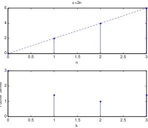
2.5 Examples of signal operations 21
3 Time-domain Analysis 25
3.1 Linear time-invariant (LTI) systems 25
3.2 Difference equations 26
3.3 Block diagram for LTI systems 28
www.sylvania.com
We do not reinvent
the wheel we reinvent
light.
Fascinating lighting offers an infinite spectrum of possibilities: Innovative technologies and new markets provide both opportunities and challenges. An environment in which your expertise is in high demand. Enjoy the supportive working atmosphere within our global group and benefit from international career paths. Implement sustainable ideas in close cooperation with other specialists and contribute to influencing our future. Come and join us in reinventing light every day.
Download free eBooks at bookboon.com
Click on the ad to read more
5
3.4 Impulse response 29
3.5 Convolution 33
3.6 Graphically demonstrated convolution 38
4 Frequency Domain Analysis 42
4.1 Fourier series for periodic digital signals 42
4.2 Fourier transform for non-periodic signals 46
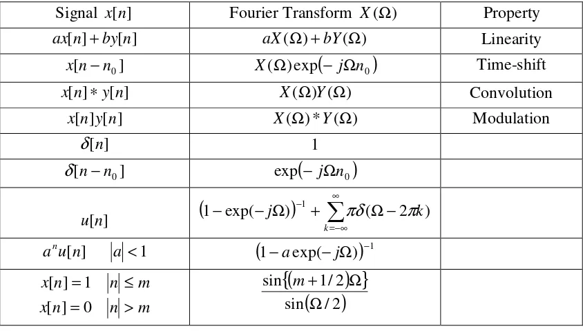
4.3 Properties of Fourier transform 49
4.4 Frequency response 50
4.5 Frequency correspondence when sampling rate is given 56
5 Z Domain Analysis 60
5.1 z-transform and inverse z-transform 60
5.2 Relationship between z-transform and Fourier transform 62
5.3 Z as time shift operator 62
5.4 Transfer function 63
5.5 Z-plane, poles and zeros 67
5.6 Stability of a system 71
5.7 Evaluation of the Fourier transform in the z-plane 75
5.8 Characteristics of 1st and 2nd order systems 77
6 Discrete Fourier Transform 88
6.1 Definition of discrete Fourier transform 88
EADSunites a leading aircraft manufacturer, the world’s largest helicopter supplier, a global leader in space programmes and a worldwide leader in global security solutions and systems to form Europe’s largest defence and aerospace group. More than 140,000 people work at Airbus, Astrium, Cassidian and Eurocopter,
in 90 locations globally, to deliver some of the industry’s most exciting projects.
An EADS internship offers the chance to use your theoretical knowledge and apply it first-hand to real situations and assignments during your studies. Given a high level of responsibility, plenty of
learning and development opportunities, and all the support you need, you will tackle interesting challenges on state-of-the-art products.
We welcome more than 5,000 interns every year across disciplines ranging from engineering, IT, procurement and finance, to strategy, customer support, marketing and sales. Positions are available in France, Germany, Spain and the UK.
To find out more and apply, visit www.jobs.eads.com. You can also find out more on our EADS Careers Facebookpage.
Download free eBooks at bookboon.com
Click on the ad to read more
6
6.2 Properties of DFT 90
6.3 The fast Fourier transform (FFT) 93
7 Spectral Analysis by DFT 100
7.4 Digital spectral analysis 100
7.5 Spectra of harmonics 100
7.6 Spectral leakage 102
7.4 Windowing 104
9.8 Performance of windows 104
7.6 Applications of digital spectral analysis 107
8 Summary 110
Bibliography 111
360°
thinking
.
© Deloitte & Touche LLP and affiliated entities.
Download free eBooks at bookboon.com
7
Preface
Since the 1990s, digital signals have been increasingly used not only in various industries and engineering equipments but also in everybody’s daily necessities. Mobile phones, TV receivers, music CDs, multimedia computing, etc, are the indispensable items in modern life, in which digital formats are taken as a basic form for carrying and storing information. The major reason for the advancement in the use of digital signals is the big leap forward in the popularization of microelectronics and computing technology in the past three decades. Traditional analogue broadcast is being widely upgraded to digital. A general shift from analogue to digital systems has taken place and achieved unequivocal benefits in signal quality, transmission efficiency and storage integrity. In addition, data management advantage in digital systems has provided users with a very friendly interface. A typical example is the popular pull-down manual, easy to find, make choices and more choices are made available.
As marching into the digital era, many people in different sectors are quite keen to understand why this has happened and what might be the next in this area. They hope to obtain basic principles about digital signals and associated digital systems. Instead of targeting advanced or expert level, they as beginners often hope to grasp the subject as efficient and effective as possible without undertaking impossible task under usually limited time and effort available.
This book is written for those beginners who want to gain an overview of the topic, understand the basic methods and know how to deal with basic digital signals and digital systems. No matter the incentive is from curiosity, interest or urgently acquiring needed knowledge for one’s profession, this book is well suited. The output standards are equivalent to university year two which lays a good foundation for further studies or moving on to specialised topics, such as digital filters, digital communications, discrete time-frequency representation, and time-scale analysis. The required mathematics for the reader is basically at pre-university level, actually only junior high schools maths is mainly involved. The content of materials in this book has been delivered to second year engineering and IT students at university for more than 10 years. A feature in this book is that the digital signal or system is mainly treated as originally existing in digital form rather than always regarded as an approximation version of a corresponding analogue system which gives a wrong impression that digital signal is poor in accuracy, although many digital signals come from taking samples out of analogue signals. The digital signal and system stand as their own and no need to use the analogue counter part to explain how they work.
To help understanding and gaining good familiarity to the topic, it will be very helpful to do some exercises attached to each chapter, which are selected from many and rather minimal in term of work load.
Weiji Wang
Download free eBooks at bookboon.com
8
1 Digital Signals and Sampling
1.1 Introduction
Digital signal processing (DSP) has become a common tool for many disciplines. The topic includes the methods of dealing with digital signals and digital systems. The techniques are useful for all the branches of natural and social sciences which involve data acquisition, analysis and management, such as engineering, physics, chemistry, meteorology, information systems, financial and social services. Before the digital era, signal processing devices were dominated by analogue type. The major reason for DSP advancement and shift from analogue is the extraordinary growth and popularization of digital microelectronics and computing technology.
The reason that digital becomes a trend to replace analogue systems, apart from it is a format that microprocessors can be easily used to carry out functions, high quality data storage, transmission and sophisticated data management are the other advantages. In addition, only 0s and 1s are used to represent a digital signal, noise can easily be suppressed or removed. The quality of reproduction is high and independent of the medium used or the number of reproduction. Digital images are two dimensional digital signals, which represent another wide application of digital signals. Digital machine vision, photographing and videoing are already widely used in various areas.
In the field of signal processing, a signal is defined as a quantity which carries information. An analogue signal is a signal represented by a continuous varying quantity. A digital signal is a signal represented by a sequence of discrete values of a quantity. The digital signal is the only form for which the modern microprocessor can take and exercise its powerful functions. Examples of digital signals which are in common use include digital sound and imaging, digital television, digital communications, audio and video devices.
To process a signal is to make numerical manipulation for signal samples. The objective of processing a signal can be to detect the trend, to extract a wanted signal from a mixture of various signal components including unwanted noise, to look at the patterns present in a signal for understanding underlying physical processes in the real world. To analyse a digital system is to find out the relationship between input and output, or to design a processor with pre-defined functions, such as filtering and amplifying under applied certain frequency range requirements. A digital signal or a digital system can be analysed in time domain, frequency domain or complex domain, etc.
1.2
Signal representation and processing
Representation of digital signals can be specific or generic. A digital signal is refereed to a series of numerical numbers, such as:
…, 2, 4, 6, 8, …
Download free eBooks at bookboon.com
9
...
],
2
[
],
1
[
],
0
[
],
1
[
...,
x
−
x
x
x
where -1, 0, 1, 2 etc are the sample numbers, x[0], x[1], x[2], etc are samples. The square brackets represent the digital form. The signal can be represented as a compact form
∞
<
<
∞
−
n
n
x
[
]
(1.1)
In the signal, x[-1], x[1], x[100], etc, are the samples,
n
is the sample number. The values of a digital signal are only being defined at the sample number variablen
, which indicates the occurrence order of samples and may be given a specific unit of time, such as second, hour, year or even century, in specific applications.We can have many digital signal examples:
- Midday temperature at Brighton city, measured on successive days, - Daily share price,
- Monthly cost in telephone bills, - Student number enrolled on a course, - Numbers of vehicles passing a bridge, etc.
Examples of digital signal processing can be given in the following:
Example 1.1 To obtain a past 7 day’s average temperature sequence. The averaged temperature sequence for past 7 days is
(
[
]
[
1
]
[
2
]...
[
6
]
)
7
1
]
[
n
=
x
n
+
x
n
−
+
x
n
−
+
x
n
−
y
.For example, if n=0 represents today, the past 7 days average is
(
[
0
]
[
1
]
[
2
]...
[
6
]
)
7
1
]
0
[
=
x
+
x
−
+
x
−
+
x
−
y
where
x
[
0
],
x
[
−
1
],
x
[
−
2
],
...
represent the temperatures of today, yesterday, the day before yesterday, …;y
[
0
]
represents the average of past 7 days temperature from today and including today. On the other hand,
(
[
1
]
[
0
]
[
1
]
...
[
5
]
)
7
1
]
1
[
=
x
+
x
+
x
−
+
+
x
−
y
Download free eBooks at bookboon.com
10
∑
=+
−
=
71
]
1
[
7
1
]
[
k
k
n
x
n
y
where x[n] is the temperature sequence signal and y[n] is the new averaged temperature sequence. The purpose of average can be used to indicate the trend. The averaging acts as a low-pass filter, in which fast fluctuations have been removed as a result. Therefore, the sequence y[n] will be smoother than x[n].
Example 1.2. To obtain the past M day simple moving averages of share prices, let x[n] denotes the close price,
y
M[
n
]
the averaged close price over past M days.
(
[
]
[
1
]
[
2
]...
[
1
]
)
1
]
[
=
x
n
+
x
n
−
+
x
n
−
+
x
n
−
M
+
M
n
y
Mor
∑
=+
−
=
Mk
M
x
n
k
M
n
y
1
]
1
[
1
]
[
(1.2)
For example, M=20 day simple moving average is used to indicate 20 day trend of a share price. M=5, 120, 250 (trading days) are usually used for indicating 1 week, half year and one year trends, respectively. Figure 1.1 shows a share’s prices with moving averages of different trading days.
Download free eBooks at bookboon.com
11
1.3
Analogue-to-digital conversion
Although some signals are originally digital, such as population data, number of vehicles and share prices, many practical signals start off in analogue form. They are continuous signals, such as human’s blood pressure, temperature and heart pulses. A continuous signal can be first converted to a proportional voltage waveform by a suitable transducer, i.e. the analogue signal is generated. Then, for adapting digital processor, the signal has to be converted into digital form by taking samples. Those samples are usually equally spaced in time for easy processing and interpretation. Figure 1.2 shows a analogue signal and its digital signal by sampling with equal time intervals. The upper is the analogue signal x(t) and the lower is the digital signal sampled at time t = nT, where n is the sample number and T is the sampling interval. Therefore,
)
(
]
[
n
x
nT
x
=
0 20 40 60 80 100 -50
0 50
t
0 20 40 60 80 100 -50
0 50
t
Figure 1.2 An analogue signal x(t) and digital signal x[n]. The upper is the analogue signal and the lower is the digital signal sampled at t = nT.
1.4
Sampling theorem
Download free eBooks at bookboon.com
Click on the ad to read more
12 - Shannon’s sampling theorem
Claude E. Shannon 1916-1949)established the sampling theorem that an analogue signal containing components up to maximum frequency
f
c Hz may be completely represented by samples, provided that the sampling ratef
s is at least 2f
c (i.e. at least 2 samples are to present per period). That isc
s
f
f
≥
2
(1.3)
Let the sampling interval
s
f
T
=
1
, the sampling requirement is equivalently represented asc
f
T
2
1
≤
(1.4)Given sampling frequency
f
s, the maximum analogue frequency allowed in the signal isT
f
f
c s2
1
2
1
=
=
(1.5)Under sampling will cause aliasing. That is, details of original signal will be lost and high frequency waveforms may be mistakenly represented as low frequency ones by the sampled digital signal. See Figure 1.3. It is worth noting that use of minimum sampling frequency is not absolutely safe, as those samples may just been placed at all zeros-crossing points of the waveform.
We will turn your CV into
an opportunity of a lifetime
Do you like cars? Would you like to be a part of a successful brand? We will appreciate and reward both your enthusiasm and talent. Send us your CV. You will be surprised where it can take you.
Download free eBooks at bookboon.com
13 Example 1.3 An analogue signal is given as
t
t
t
t
t
x
(
)
=
sin
3000
+
2
cos
350
+
sin
200
cos
20
where t is the time in seconds, determine the required minimum sampling frequency for the signal and calculate the time interval between any two adjacent samples.
Solution:
The third term is equivalent to 2 components of frequencies 200+20 hz and 200-20 hz. The highest frequency in the
signal therefore is
3000
/
2
π
=
477
.
5
hz
. Required minimum sampling frequency is2
×
477
.
5
hz
=
955
hz
,
, orthe sampling interval T is
1
/
955
=
0
.
001047
seconds
.0 200 400 600 800 1000
-2 0 2
Ov
er
sa
mp
le
d
0 200 400 600 800 1000
-2 0 2
"J
us
t
ri
gh
t"
0 200 400 600 800 1000
-2 0 2
Un
der
samp
le
d
Figure 1.3 Over sampling and under sampling
1.5
Quantization in an analogue-to-digital converter
The quality of a digital signal is dependent on the quality of the conversion processes. An analogue signal takes on a continuous range of amplitudes. However, a practical electronic analogue-to-digital converter has limited levels of quantization. An n-bit analogue-to-digital converter has
2
n levels, i.e. only as many as2
n different values can be presented in the sampling.Download free eBooks at bookboon.com
14
During an unlimited level of analogue signal being converted into a limited level of digital signal, all possible values have to be rounded to those limited
2
n levels. This means a quantization error (or equivalently termed as quantization noise) has been introduced. In practice, n in the2
n needs to be chosen to be big enough to satisfy the quantization accuracy. When n=3,2
n=8 provides 8 quantization levels. Obviously, there exists big quantization errors in representing the original continuous signal by a small number of levels. But when taking n=12, it gives as many as 4096 quantization levels, which satisfies many industrial applications.The following Figure 1.4 illustrates the quantization process in which the analogue to digital convertor has 8 levels. A continuous signal is sampled to a digital signal as …,1, 6, 6, 5, 5, 4, 4, 4, 4, 6,… which have difference, i.e. the error, at each sampling point between the analogue and digital values.
7
6
5
4
3
2
1
1 2 3 4 5 6 7 8 9
10
n
Figure 1.4 Continuous signal is sampled as 8 levels of digital signal.
Problems
Q1.1 Observe the signals in Fig. Q1.1 and answer the following questions:
a) What is the frequency of the analogue sinusoidal signal (solid line) ? _______.
b) How many samples have been taken from the analogue signal within one second (the sampling frequency)? ________.
c) Does the digital signal (the dotted line) represent the original analogue signal correctly? _________ . What has happened? _____________________.
d) What is the frequency of the digital sinusoidal signal? ______.
Download free eBooks at bookboon.com
15
0 0.2 0.4 0.6 0.8 1
- 2 -1.5
- 1 -0.5
0 0.5
1 1.5
2
seconds x
Figure Q1.1
Q1.2 A stock price can be described by a digital series
x
[
n
]
, where n indicates the day: -∞<n<∞. The past M day (including the present day) simple moving average (SMA) series is often used for trend analysis.Download free eBooks at bookboon.com
Click on the ad to read more
16
2 Basic Types of Digital Signals
2.1
Three basic signals
Unit impulse
≠
=
=
0
0
0
1
]
[
n
n
n
d
(2.1)i.e. the unit impulse has only one non-zero value 1 at n=0, and all other samples are 0. It is the simplest signal but will be seen later very important.
Unit step
<
≥
=
0
0
0
1
]
[
n
n
n
u
(2.2)
where the sample value rises at n=0 from 0 to 1 and keeps it to
n
→
∞
.Ramp
as a
e
s
al na
or o
eal responsibili�
I joined MITAS because
Maersk.com/Mitas�e Graduate Programme for Engineers and Geoscientists
as a
e
s
al na
or o
Month 16
I was a construction
supervisor in
the North Sea
advising and
helping foremen
solve problems
I was a
he
s
Real work International opportunities �ree work placements
al Internationa
or �ree wo
al na
or o
I wanted
real responsibili�
I joined MITAS because
Download free eBooks at bookboon.com
17
<
≥
=
0
0
0
]
[
n
n
n
n
r
(2.3)
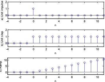
Figure 2.1 illustrates the unit impulse, unit step and ramp signals. Alternatively, the three basic signals can be expressed by a tabular form as below:
n
…
-3
-2
-1
0
1
2
3
…
d[n]
…
0
0
0
1
0
0
0
. . .
u[n]
…
0
0
0
1
1
1
1
…
r[n]
…
0
0
0
0
1
2
3
…
Download free eBooks at bookboon.com
18
-4 -2 0 2 4 6 8 10
0 1 2
a)
U
ni
t i
m
pul
s
e
n
-4 -2 0 2 4 6 8 10
0 1 2
b)
U
ni
t s
tep
n
-4 -2 0 2 4 6 8 10
0 5 10
c
) Ra
m
p
n
Figure 2.1 Unit impulse, unit step and ramp signals
2.2
Other basic signals
- Sinusoidal signals
Sinusoidal signals are referred to the sine and cosine functions. In digital format, they are
)
sin(
]
[
)
cos(
]
[
W
=
W
=
n
A
n
x
n
A
n
x
(2.4)
where, it is worth noting,
W
is the frequency with a unit of radians/sample, n is the sample number. The sinusoidal functions have a period of2
p
.- Exponential signal
n
Ae n x[ ]= β
or
)
exp(
]
[
n
A
n
x
=
β
Download free eBooks at bookboon.com
Click on the ad to read more
19 where A, βare constants and n the sample number.
- Complex signals z
A digital signal x[n] can be complex, a simple example is
)
sin(
)
cos(
]
[
n
=
n
W
+
j
n
W
x
where
j
=
−
1
, and the signal has real and imaginary parts. Note that according to Euler formula(
jn
Ω
)
=
cos
(
n
Ω
)
+
j
sin
(
n
Ω
)
exp
, t
, there are relationships:)}
exp(
)
{exp(
2
1
)
sin(
)}
exp(
)
{exp(
2
1
)
cos(
W
−
−
W
=
W
W
−
+
W
=
W
jn
jn
j
n
jn
jn
n
Download free eBooks at bookboon.com
20
2.3
Signal shifting, flipping and scaling
- Signal shifting
A signal can be shifted to left or right by any number of samples. In Figure 2.2 (a), a unit impulse has been shifted to the
right by one sample; and in Figure 2.2 (b), a unit impulse
d
[
n
]
has been shifted to the left by one sample. They shouldbe represented by
d
[
n
−
1
]
(shifted to the right) andd
[
n
+
1
]
(shifted to the left), respectively. For the general case ofa signal
x
[
n
]
, shifting to the right and left byn
0samples generates new signalsx
[
n
−
n
0]
andx
[
n
+
n
0]
. They are adelayed signal and an advanced signal, respectively.
1 0
n
-1 0
n
(a) (b)
Figure 2.2 Unit impulse is shifted to left: d[n+1] (a) and Shifted to right: d[n-1] (b)
- Signal flipping
A unit step
u
[
n
]
flipped about y-axis can generate a new signalu
[
−
n
]
shown in Figure 2.3(a). It can also be flippedand then shifted to left by one sample as
u
[
−
(
n
+
1
)]
oru
[
−
n
−
1
]
as shown in Figure 2.3(b). In general cases, a flipped signal ofx
[
n
]
isx
[
−
n
]
.0
n n
0 -1
(a) (b)
Figure2.3 Unit step is flipped as u[-n] (a) and shifted to the left: u[-n-1] = u[-(n+1)] (b)
Download free eBooks at bookboon.com
21
In Figure 2.4, a shifted unit impulse
d
[
n
−
1
]
is been scaled by -2 to -2d
[
n
−
1
]
. For general cases, a signalx
[
n
]
scaled by numbera
isax
[
n
]
.0
n 1
-2
Figure 2.4 A shifted unit impulse is being scaled by -2.
2.4
Periodic signals
A periodic signal satisfies the following relationship
]
[
]
[
n
kN
x
n
x
±
=
(2.7)
where k is an arbitrary integer and N the period. The above relationship indicates that a periodic signal can remain the same shape if it shifts to left or right by any integer number of periods. Typical periodic signals are sine and cosine waves.
e.g. For the signal
=
1
1
sin
]
[
n
n
p
x
, we can find the period by following steps:We know that the sine function has a period of
2
p
. Therefore,
±
=
±
=
1
1
)
2
2
(
sin
2
1
1
sin
1
1
sin
n
p
n
p
p
n
p
This means that on the n-axis, a new signal after being shifted to left or right by 22 samples is still identical to the original signal. Therefore, N=22 (samples)is the period.
2.5
Examples of signal operations
For 6 signals in Figure 2.5, the expressions using basic signals, including the unit impulse, unit step and ramp, can be found as
a) x[n]=-2 u[n] b) x[n]=-5 u[-n-4] c) x[n]= u[n+3] - u[n-5] d) x[n]= 5 d[n-6]
Download free eBooks at bookboon.com
Click on the ad to read more
22
In b), the signal has been flipped, scaled by -5 and shifted to the left by 4 samples
−
5
u
[
−
n
−
4
]
=
−
5
u
[
−
(
n
+
4
)]
.
. c) is an rectangular function or a window function. In f) the gradient has been changed by scaling factor 2.-5 0 5 10 -2
0 2
(a
)
-10 -5 0 5 -10
0 10
(b
)
-5 0 5 -2
0 2
(c
)
-5 0 5 10 -10
0 10
(d
)
-5 0 5 10 -2
0 2
(e
)
-5 0 5 -10
0 10
(f
)
Figure 2.5 Examples of signal operations
Download free eBooks at bookboon.com 23
¦
¦
−∞ = ∞ ==
−
=
+
−
+
−
+
=
n m km
k
n
n
n
n
n
u
[
]
[
]
[
1
]
[
2
]
...
[
]
[
]
0
δ
δ
δ
δ
δ
(2.8)And, the unit impulse can be represented by the unit steps as
]
[
]
[
]
[
]
[
]
[
]
[
]
1
[
]
[
1 1 1n
m
m
n
m
m
n
u
n
u
n m n m n m n mδ
δ
δ
δ
δ
δ
−
=
+
−
=
=
−
−
¦
¦
¦
¦
− −∞ = − −∞ = − −∞ = −∞ =i.e. the impulse response is the difference of two unit steps.
]
1
[
]
[
]
[
n
=
u
n
−
u
n
−
d
. (2.9)Problems
Q2.1 Sketch and label the following digital signals
a)
−
u
[
n
+
1
]
b)u
[
−
n
+
1
]
c)
u
[
n
+
2
]
+
2
d
[
n
−
3
]
d)
3
u
[
n
+
4
]
−
3
u
[
n
−
5
]
e)
r
[
n
+
1
]
−
2
r
[
n
−
2
]
Q2.2 Sketch and label the digital signal
a)
2
sin
]
[
1
]
[
u
n
n
n
n
x
=
p
b)
x
[
n
]
=
u
[
n
+
2
]
−
u
[
n
−
3
]
+
r
[
n
−
3
]
−
r
[
n
−
6
]
+
2
d
[
n
]
where
d
[
n
]
,
u
[
n
]
and
r
[
n
]
are the unit impulse, unit step and ramp functions, respectively.Q2.3 Let
d
[
n
],
u
[
n
]
and
r
[
n
]
be the unit impulse, unit step and ramp functions, respectively. Given]
5
[
]
4
[
]
2
[
]
[
]
[
]
[
]
6
[
]
[
]
[
2 1−
−
−
−
−
+
+
=
−
−
=
n
r
n
n
n
n
r
n
x
n
u
n
u
n
x
d
d
d
Download free eBooks at bookboon.com
24
Q2.4 Let
d
[
n
],
u
[
n
]
and
r
[
n
]
be the unit impulse, unit step and ramp functions, respectively. Given]
[
]
2
[
]
[
]
4
[
]
2
[
]
[
2 1
n
n
r
n
x
n
u
n
u
n
x
d
−
−
=
−
−
−
=
Sketch and label the digital signals
x
1[
n
]
+
x
2[
n
]
andx
1[
n
]
⋅
x
2[
n
]
.Q2.5 Find the period of the following digital signal:
(a)
11
sin
]
[
n
n
x
π
=
(b)
¸¸
¹
·
¨¨
©
§
−
+
¸¸
¹
·
¨¨
©
§
+
=
π
π
π
π
15
2
cos
3
sin
3
]
[
n
n
n
x
(c)
15
2
cos
6
sin
4
3
sin
3
2
]
[
n
n
n
n
x
π
π
π
+
+
+
=
.
Q2.6 Two pperiodic digital signals are given as
23
2
sin
]
[
,
16
cos
1
]
[
21
n
n
x
n
n
x
π
π
=
+
=
Download free eBooks at bookboon.com
Click on the ad to read more
25
3 Time-domain Analysis
3.1
Linear time-invariant (LTI) systems
A digital system is also refereed as a digital processor, which is capable of carrying out a DSP function or operation. The digital system takes variety of forms, such as a microprocessor, a programmed general-purpose computer, a part of digital device or a piece of computing software.
Among digital systems, linear time-invariant (LTI) systems are basic and common. For those reasons, it will be restricted to address about only the LTI systems in this whole book.
The linearity is an important and realistic assumption in dealing with a large number of digital systems, which satisfies
the following relationships between input and output described by Figure 3.1. i.e. a single input
x
1[
n
]
produces a singleoutput
y
1[
n
]
, Applying sum of inputsx
1[
n
]
+
x
2[
n
]
producesy
1[
n
]
+
y
2[
n
]
, and applying inputax
1[
n
]
+
bx
2[
n
]
Download free eBooks at bookboon.com
26
Linear System
Input
Output
x
1[
n
]
y
1[
n
]
]
[
1
n
ax
ay
1[
n
]
]
[
2
n
x
y
2[
n
]
x
1[
n
]
+
x
2[
n
]
y
1[
n
]
+
y
2[
n
]
]
[
]
[
21
n
bx
n
ax
+
ay
1[
n
]
+
by
2[
n
]
Figure 3.1 Linearity of a system
The linearity can be described as the combination of a scaling rule and a superposition rule. The time-invariance requires the function of the system does not vary with the time. e.g. a cash register at a supermarket adds all costs of purchased items
x
[
n
]
,x
[
n
−
1
]
,… at check-out during the period of interest, and the total costy
[
n
]
is given by...
]
2
[
]
1
[
]
[
]
[
n
=
x
n
+
x
n
−
+
x
n
−
+
y
(3.1)where
y
[
n
]
is the total cost, and ifx
[
0
]
is an item registered at this moment,x
[
−
1
]
then is the item at the last moment, etc. The calculation method as a simple sum of all those item’s costs is assumed to remain invariant at the supermarket, at least, for the period of interest.3.2
Difference equations
Like a differential equation is used to describe the relationship between its input and output of a continuous system, a difference equation can be used to characterise the relationship between the input and output of a digital system. Many systems in real life can be described by a continuous form of differential equations. When a differential equation takes a discrete form, it generates a difference equation. For example, a first order differential equation is commonly a mathematical model for describing a heater’s rising temperature, water level drop of a leaking tank, etc:
)
(
)
(
)
(
t
bx
t
ay
dt
t
dy
=
+
(3.2)
where
x
[
n
]
is the input andy
[
n
]
is the output. For digital case, the derivative can be described asT n y n y dt
t
dy() [ ]− [ −1]
= ,
(3.3)
Download free eBooks at bookboon.com 27 ] [ ] [ ] 1 [ ] [ n bx n ay T n y n y = + − − or
]
[
]
1
[
]
[
)
1
(
+
Ta
y
n
=
y
n
−
+
Tbx
n
yielding a standard form difference equation:
]
[
]
1
[
]
[
n
a
1y
n
b
1x
n
y
=
−
+
(3.4)where
Ta
a
+
=
1
1
1
a
andTa
Tb
b
+
=
1
1 are constants.
For input’s derivative, we have similar digital form as
T
n
x
n
x
dt
t
dx
(
)
[
]
−
[
−
1
]
=
.
.
Further, the second order derivative in a differential equation contains can be discretised as
2 2 ) ( dt t y
d
(
)
] 2 [ ] 1 [ 2 ] [ 1 ] 2 [ ] 1 [ ] 1 [ ] [
2 − − + −
= − − − − − −
= y n yn yn
T T T n y n y T n y n y
. (3.5)
When the output can be expressed only by the input and shifted input, the difference equation is called non-recursive equation, such as
]
2
[
]
1
[
]
[
]
[
n
=
b
1x
n
+
b
2x
n
−
+
b
3x
n
−
y
(3.6)
On the other hand, if the output is expressed by the shifted output, the difference equation is a recursive equation, such as
]
3
[
]
2
[
]
1
[
]
[
n
=
a
1y
n
−
+
a
2y
n
−
+
a
3y
n
−
y
(3.7)
where the output
y
[
n
]
is expressed by it shifted signalsy
[
n
−
1
]
,y
[
n
−
2
]
, etc. In general, an LTI processor can be represented as...
]
2
[
]
1
[
...
]
2
[
]
1
[
]
[
n
=
a
1y
n
−
+
a
2y
n
−
+
+
b
1x
n
−
+
b
2x
n
−
+
y
or a short form
]
[
]
[
]
[
0 1k
n
x
b
k
n
y
a
n
y
k M k k N k−
+
−
=
∑
∑
=Download free eBooks at bookboon.com
Click on the ad to read more
28 or
∑
∑
= =
−
=
−
Mk k N
k
k
y
n
k
b
x
n
k
a
0 0
'
[
]
[
]
(3.9)
A difference equation is not necessarily from the digitization of differential equation. It can originally take digital form, such as the difference equation in Eq.(3.1).
3.3
Block diagram for LTI systems
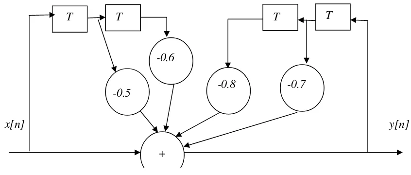
Alternatively, equivalent to the difference equation, an LTI system can also be represented by a block diagram, which also characterises the input and output relationship for the system.
For example, to draw a block diagram for the digital system described by the difference equation:
]
2
[
6
.
0
]
1
[
5
.
0
]
[
]
2
[
8
.
0
]
1
[
7
.
0
]
[
n
+
y
n
−
+
y
n
−
=
x
n
−
x
n
−
−
x
n
−
y
The output can be rewrite as
]
2
[
6
.
0
]
1
[
5
.
0
]
[
]
2
[
8
.
0
]
1
[
7
.
0
]
[
n
=
−
y
n
−
−
y
n
−
+
x
n
−
x
n
−
−
x
n
−
y
The block diagram for the system is shown in Figure 3.2.
“The perfect start
of a successful,
international career.”
CLICK HERE
to discover why both socially and academically the Universityof Groningen is one of the best places for a student to be
www.rug.nl/feb/education
Download free eBooks at bookboon.com
29
In the bock diagram, T is the sampling interval, which acts as a delay or right-shift by one sample in time. For general cases, instead of Eq.(3.9), Eq. (3.8) is used for drawing a block diagram. It can easily begin with the input, output flows and the summation operator, then add input and output branches.
+
x[n]
y[n]
-0.5
-0.6
-0.7
-0.8
T
T
T
T
Figure 3.2 Block diagram of an LTI system
3.4
Impulse response
Both the difference equation and block diagram can be used to describe a digital system. Furthermore, the impulse response can also be used to represent the relationship between input and output of a digital system. As the terms suggest, impulse response is the response to the simplest input – unit impulse. Figure 3.2 illustrates a digital LTI system, in which the input is the unit impulse and the output is the impulse response.
δ
[n]
h[n]
Digital LTI system
Figure 3.2 Unit impulse and impulse response
Input d[n] Output h[n]
0 n n
Figure 3.3 Unit impulse and impulse response of a causal system
Once the impulse response of a system is known, it can be expected that the response to other types of input can be derived.
Download free eBooks at bookboon.com
30
Input d[n] Output h[n]
0 n n
Figure 3.4 Unit impulse and impulse response of a non-causal system
The impulse response of a system can be evaluated from its difference equation. Following are the examples of finding the values of impulse responses from difference equations
Example 3.1 Evaluating the impulse response for the following systems
a) y[n]=3 x[n] + x[n-1] + 4 x[n-2]
We know that when the input is the simplest unit impulse d[n], the output response will be the impulse response. Therefore, replacing input x[n] by d[n] and response y[n] by h[n], the equation is still holding and has become special:
h[n]=3 d[n] + d[n-1] + 4 d[n-2]
It is easy to evaluate the impulse response by letting n=-1, 0,1,2,3,…
When n=-1, h[-1]=0
When n=0, h[0]= 3 d[0] +d[-1] + 4 d[-2]=3 When n=1, h[1]= 1,
When n=2, h[2]= 4, When n=3, h[3]= 0, …
Therefore, the impulse response h[n]=[3, 1, 4, 0, …] ↑
where ↑indicates the position of origin n=0.
b) Assume the system is causal. With the difference equation
y[n]=1.5 y[n-1] -0.85 y[n-2] + x[n]
We have
Download free eBooks at bookboon.com
Click on the ad to read more
31 Let n=0, 1, 2, 3,…
h[0]=0-0+1=1 h[1]=1.5 ´1-0 -0=1.5 h[2]=1.5´1.5-0.85´1+0=1.4 h[3]=1.5´1.4-0.85´1.5+0 =0.825 ...
Therefore, the impulse response h[n]=[1, 1.5, 1.4, 0.825, …]. ↑
Generally for the difference equation:
...
]
3
[
]
2
[
]
1
[
...
]
3
[
]
2
[
]
1
[
]
[
n
=
a
1y
n
−
+
a
2y
n
−
+
a
3y
n
−
+
+
b
1x
n
−
+
b
2x
n
−
+
b
3x
n
−
+
y
The impulse response can evaluated by the special equation with the simple unit impulse input:
...
]
2
[
]
1
[
...
]
2
[
]
1
[
]
[
n
=
a
1h
n
−
+
a
2h
n
−
+
+
b
1n
−
+
b
2n
−
+
h
d
d
(3.10)
Download free eBooks at bookboon.com
32
The step response is also commonly used to characterize the relationship between the input and output of a system. To find the step response using the impulse response, we know that the unit step can be expressed by unit impulses as
...
]
2
[
]
1
[
]
[
]
[
n
=
n
+
n
−
+
n
−
+
u
d
d
d
(3.11)The linear system satisfies the superposition rule. Therefore, the step response is a sum of a series of impulse responses excited by a series of shifted unit impulses. i.e., the step responseis a sum of impulse responses
∑
∑
−∞ = ∞
=
=
−
=
+
−
+
−
+
=
nm k
m
h
k
n
h
n
h
n
h
n
h
n
s
[
]
[
]
[
1
]
[
2
]
...
[
]
[
]
0 (3.12)
To better understand Eq. (3.12), we can make use of the linearity of the LTI systems. In Figure 3.5, it has been shown that the input is decomposed in to impulses according to Eq.(3.11), and the output is the responses of all individual impulse responses described in Eq. (3.12).
]
[
...
...
]
2
[
]
1
[
]
1
[
]
2
[
]
[
]
[
]
[
s
n
n
h
n
n
h
n
n
h
n
n
u
=
°
°
¿
°°
¾
½
°
°
¯
°°
®
→
→
−
→
→
−
−
→
→
−
→
→
=
δ
δ
δ
LTI System
Figure 3.5 Multiple unit impulse inputs to an LTI system
Example 3.2: Find the step response s[n] for a system described by
y[n]=0.6y[n-1] +x[n].
Solution: From the difference equation, h[n]=0.6h[n-1]+d[n], the samples of impulse response can be evaluated as
h[0]=0+1=1 h[1]=0.6´1+0=0.6 h[2]=0.6´0.6+0=0.6´0.6 h[3]=0.6´0.6´0.6+0=0.6´0.6´0.6 ...
The samples of step response are
s[0]=h[0]=1
s[1]=h[0]+h[1]=1+0.6
Download free eBooks at bookboon.com
33 s[3]= h[0]+h[1]+h[2]+h[3]=1+0.6+0.6´0.6+0.6´0.6´0.6
s[∞]=1+0.6+0.6´0.6+0.6´0.6´0.6+…
2
.
5
6
.
0
1
1
=
−
=
,where the following series summation formula is applied.
1
1
1
...
1
2 3<
−
=
+
+
+
+
a
a
a
a
a
(3.13)
3.5 Convolution
In order to derive the convolution formula based on clear understanding, a signal is expressed by impulse functions as following:
For a signal x[n], −∞ <n<∞, using the rules of the signal shifting and scaling described Section 2.3, it is decomposed into a series of unit impulses scaled by the sample values:
...
]
2
[
]
2
[
]
1
[
]
1
[
]
[
]
0
[
]
1
[
]
1
[
]
2
[
]
2
[
...
]
[
n
=
+
x
−
n
+
+
x
−
n
+
+
x
n
+
x
n
−
+
x
n
−
+
x
d
d
d
d
d
or
∑
∞−∞ =
−
=
k
k
n
k
x
n
x
[
]
[
]
d
[
]
(3.14)
The above expression can be illustrated as following. For example, a signal
x
[
n
]
has 2 non-zero samples, which can be represented as a sum of shifted and scaled unit impulsesx
[
1
]
d
[
n
−
1
]
+
x
[
2
]
d
[
n
−
2
]
, as illustrated in Figure 3.6.X[n]
=
+
0 1 2 0 1 2 0 1 2 X[2]d[n-2] X[1]d[n-1]
Figure 3.6 A signal can be decomposed into simple sequences. (Except those non-zero samples, all other samples have zero values.)
In general cases, assuming the system is causal, if the input x[n] is
Download free eBooks at bookboon.com
Click on the ad to read more
34 h[n]: ... 0 0 0 h[0] h[1] h[2] ...
↑
Then, the output y[n]is h[n]. On the other hand, if the input is x[0]d[n]: ... 0 x[0] 0 0 ... The, the output y[n] is x[0]h[n] Finally, if the input is
x[n]: ... x[-1] x[0] x[1] x[2] ... ↑
Using the linearity again, the output y[n] will be a sum of all responses to individual shifted and scaled impulses as in Eq.(3.14), shown in Figure 3.7.
www.mastersopenday.nl
Visit us and find out why we are the best!
Master’s Open Day: 22 February 2014
Join the best at
the Maastricht University
School of Business and
Economics!
Top master’s programmes
• 33rd place Financial Times worldwide ranking: MSc
International Business
• 1st place: MSc International Business
• 1st place: MSc Financial Economics
• 2nd place: MSc Management of Learning
• 2nd place: MSc Economics
• 2nd place: MSc Econometrics and Operations Research
• 2nd place: MSc Global Supply Chain Management and
Change
Sources: Keuzegids Master ranking 2013; Elsevier ‘Beste Studies’ ranking 2012; Financial Times Global Masters in Management ranking 2012
Maastricht University is the best specialist
university in the Netherlands
Download free eBooks at bookboon.com 35
]
[
...
...
]
2
[
]
2
[
]
2
[
]
2
[
]
1
[
]
1
[
]
1
[
]
1
[
]
[
]
0
[
]
[
]
0
[
]
1
[
]
1
[
]
1
[
]
1
[
...
...
]
[
y
n
n
h
x
n
x
n
h
x
n
x
n
h
x
n
x
n
h
x
n
x
n
x
=
°
°
°
°
¿
°°
°
°
¾
½
°
°
°
°
¯
°°
°
°
®
−
→
→
−
−
→
→
−
→
→
+
−
→
→
+
−
=
δ
δ
δ
δ
.
LTI
System
. Figure 3.7 Decomposed inputs generate decomposed outputs.
i.e. the output of an LTI system will be
...
]
2
[
]
2
[
]
1
[
]
1
[
]
[
]
0
[
]
1
[
]
1
[
...
]
[
n
=
+
x
−
h
n
+
+
x
h
n
+
x
h
n
−
+
x
h
n
−
+
y
(3.15)or
∑
∞ −∞ =
−
=
kk
n
h
k
x
n
y
[
]
[
]
[
]
(3.16)Eq. (3.15) or (3.16) is called the convolution sum or convolution, which describes how the input and impulse response are engaged to generate the output in an LTI system. For short, the convolution sum is also represented by
]
[
*
]
[
]
[
n
x
n
h
n
y
=
(3.17)where ‘*’ represents the convolution operation. Explicitly, the samples of the response by the convolution are
y[0]= ...+ x[-1] h[1]+ x[0] h[0]+ x[1] h[-1] + x[2] h[-2] + ...
y[1]= ...+ x[-1] h[2]+ x[0] h[1]+ x[1] h[0] + x[2] h[-1] + ... (3.18)
y[2]= ...+ x[-1] h[3]+ x[0] h[2]+ x[1] h[1] + x[2] h[0] + ... … …
Eq. (3.18) describes the way of calculating a convolution. For manually calculating the convolution, put x[n] in normal order and put h[n] in a flipped order. x[n] and h[n] are aligned with their origin. The output sample y[0] can be calculated by a sum of multiplications between corresponding samples. Shifting h’[n] right by one sample, y[1] can also be calculated by a sum of multiplications between new corresponding samples. The following is an example.
Example 3.3 Obtain the output of a system using manual convolution:
n
...
-1
0
1
2
3
4
...
x[n]
...
0
4
5
6
7
8
...
Download free eBooks at bookboon.com
36
k
-4
-3
-2
-1
0
1
2
3
4
...
x[n]
0
0
0
0
4
5
6
7
8
...
h’[n] 0.03125
0.0625
0.125
0.25
0.5
0
0
0
0
... y[0]
0.03125
0.0625
0.125
0.25
0.5
0
0
0
…y[1]
0.03125
0.0625
0.125
0.25
0.5
0
0
…y[2]
0.031
0.062
0.125
0.25
0.5
0
... y[3]
° ° °
The convolution satisfies the exchange rule. From Eq. (3.16), let r=n-k, then k=n-r. When k runs from -∞ to ∞, r runs from ∞ to -∞:
∑
∞−∞ =
−
=
r
r
h
r
n
x
n
y
[
]
[
]
[
]
or
∑
∞−∞ =
−
=
k
k
n
x
k
h
n
y
[
]
[
]
[
]
i.e.
]
[
*
]
[
]
[
n
h
n
x
n
y
=
Therefore,
]
[
*
]
[
]
[
*
]
[
]
[
n
x
n
h
n
x
n
h
n
y
=
=
(3.19)Download free eBooks at bookboon.com
Click on the ad to read more
37
]
[
*
]
[
]
[
*
]
[
2 2 11
n
x
n
x
n
x
n
x
=
(3.20)Example 3.4: A filter’s difference equation is y[n]-0.5 y[n-1]=0.5 x[n], where x[n]: ...0 0 4 5 6 7 8 9 10 ... ↑
a) Find the impulse response of the filter and to calculate samples of response y[0], y[1], ... , y[4]. b) Check y[n] can be found by the difference equation.
Solution:
a) From
y[n]=0.5 y[n-1] + 0.5 x[n]
we know
h[n]=0.5 h[n-1]+ 0.5 d[n]
Then, the impulse response can be evaluated h[0]= 0.5 ´ 1=0.5
h[1]= 0.5 ´ 0.5 =0.25 h[2]=0.5 ´ 0.25=0.125
- © Photononstop
REDEFINE
YOUR FUTURE
>
Join AXA,
Download free eBooks at bookboon.com
38 Using the manual convolution method,
y[0]=4 ×0.5=2
y[1]=4 ×0.25+5 ×0.5=3.5
y[2]=4 ×0.125+5 ×0.25+6 ×0.5=4.75
y[3]=4 ×0.0625+5 ×0.125+6 ×0.25+7 ×0.5=5.875
y[4]=4 ×0.03125+5×0.0625+6 ×0.125+7 ×0.25+7 ×0.5=6.9375
c) Direct calculation
Causality is assumed in this case …, i.e. x[-2]=0, x[-1]=0. Therefore, it can be determined
…, y[-2], y[-1]=0,
using
y[n]=0.5 y[n-1] + 0.5 x[n]
y[-1]=0
y[0]=0.5×0+0.5×4=2 y[1]= 0.5×2+0.5×5=3.5 y[2]=0.5×3.5+0.5×6=4.75 y[3]=0.5×4.75+0.5×7=5.875 y[4]=0.5×5.875+0.5×8=6.9375
3.6
Graphically demonstrated convolution
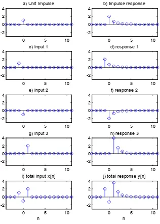
The following Figure 3.8 illustrates how the convolution between the input and impulse response is carried out.
a) and b) are the unit impulse and impulse response, respectively. c) is the input 1 : x[-1]d[n+1]. The response is in d) : h[n+1]. e) and f) are the input 2 : x[0] ]d[n] and response 2 :x[0]h[n]. g) and h) are the input 3 : x[1] ]d[n-1] and response 3 : x[1]h[n-1]. i) is the total input x[n]=… x[-1]d[n+1]+ x[0] ]d[n]+ x[1] ]d[n-1]+… j) is the total response y[n]= … x[-1]h[n+1]+ x[0] ]h[n]+ x[1] ]h[n-1]+… i.e.
∑
∞−∞ =
−
=
k
k
n
h
k
x
n
Download free eBooks at bookboon.com
39
0 5 10
-2 0 2 4
a) Unit impulse
0 5 10
-2 0 2 4
b) Impulse response
0 5 10
-2 0 2 4
c) input 1
0 5 10
-2 0 2 4
d) response 1
0 5 10
-2 0 2 4
e) input 2
0 5 10
-2 0 2 4
f) response 2
0 5 10
-2 0 2 4
g) input 3
0 5 10
-2 0 2 4
h) response 3
0 5 10
-2 0 2 4
i) total input x[n]
n
0 5 10
-2 0 2 4
j) total response y[n]
n
Figure 3.8 Graphic expression for digital convolution
Problems
Q3.1 Many systems can be described by a continuous form of first order differential equation:
)
(
)
(
)
(
)
(
t
cx
dt
t
dx
b
t
ay
dt
t
dy
+
=
+
Download free eBooks at bookboon.com
Click on the ad to read more
40 Q3.2 A second order differential equation is:
)
(
4
)
(
)
(
3
)
(
2
)
(
2 2
t
x
dt
t
dx
t
y
dt
t
dy
dt
t
dy
+
=
+
+
Derive the corresponding discrete form of difference equation if the sampling interval is T.
Q3.3 Draw a block diagram for the digital system described by the difference equation:
a)
y
[
n
]
=
0
.
7
y
[
n
−
1
]
+
x
[
n
]
−
0
.
5
x
[
n
−
1
]
b)]
2
[
55
.
0
]
[
2
]
2
[
65
.
0
]
1
[
35
.
0
]
[
n
=
y
n
−
+
y
n
−
+
x
n
−
x
n
−
y
.
Q3.4. Evaluate the impulse responses of the following filters upto n=6:
a)
y
[
n
]
=
3
y
[
n
−
1
]
+
x
[
n
]
b)y
[
n
]
=
3
y
[
n
−
1
]
+
2
x
[
n
−
2
]
c)
y
[
n
]
=
3
y
[
n
−
1
]
+
x
[
n
]
−
2
x
[
n
−
1
]
+
3
x
[
n
−
2
]
Download free eBooks at bookboon.com
41
]
[
]
2
[
25
.
0
]
1
[
5
.
0
]
[
n
y
n
y
n
x
n
y
=
−
+
−
+
Q3.6 For LTI digital systems, the output is the convolution between the input and the impulse response. Calculate the output
y
[
n
]
by manual convolution up to n=5 for the given impulse responses and inputs:a)
[
]
↑
=
2
1
3
4
...
]
[
n
h
[
]
↑
=
1
2
3
...
]
[
n
x
b)
[
]
↑
=
4
3
2
1
0
...
]
[
n
h
[
]
↑
−
=
2
1
0
...
]
[
n
x
c)
]
[
)
5
.
0
(
]
[
n
u
n
h
=
−
n↑
=
[
10
,
10
]
Download free eBooks at bookboon.com
42
4 Frequency Domain Analysis
4.1
Fourier series for periodic digital signals
Consider a periodic digital signal x[n], n=0,1,2,...,N-1, where N is the number of sample values in each period. From Euler’s complex exponential equation:
¸¸ ¹ · ¨¨ © § − ¸¸ ¹ · ¨¨ © §
=
¸¸ ¹ · ¨¨
© § −
N kn j
N kn
N kn j
π π
π 2
sin 2
cos 2
exp k=0,1,2,...,N-1 (4.1)
for each frequency k, Eq. (4.1) contains 2 sinusoidal functions in real and imaginary parts, respectively, with p/2 difference in phase. The frequencies of the functions are k=0,1,2,...,N-1. The fundamental sinusoidal function is when the frequency k=1. The other higher sinusoidal functions are called harmonics. The coefficients ofFourier Series for a digital signal can be calculated by
¦
−=
¸¸
¹
·
¨¨
©
§
−
=
10
2
exp
]
[
1
Nn k
N
kn
j
n
x
N
a
π
k=1,2,…,N-1
(4.2)
where
a
k is kth spectral coefficient, indicating the strength of the kth harmonic function. The original digital signal x[n] can be represented by its constituent harmonics as the form of discrete Fourier series:¦
−= ¸¸¹
· ¨¨
© § =
1
0
2 exp ]
[
N k
k
N kn j a n
x
π
.(4.3)
Gambar
![Figure 1.2 An analogue signal x(t) and digital signal x[n]. The upper is the analogue signal and the lower is the digital signal sampled at t = nT.](https://thumb-ap.123doks.com/thumbv2/123dok/1318258.2011253/11.595.205.433.267.485/figure-analogue-signal-digital-analogue-signal-digital-sampled.webp)

![Figure 2.2 Unit impulse is shifted to left: d[n+1] (a) and Shifted to right: d[n-1] (b)](https://thumb-ap.123doks.com/thumbv2/123dok/1318258.2011253/20.595.135.507.245.388/figure-unit-impulse-shifted-left-d-shifted-right.webp)

Dokumen terkait
Itu Populasi penelitian adalah seluruh pegawai di kantor UPPD/Samsat Delanggu yang berjumlah 30 orang responden untuk diambil sampel penelitian dengan Instrumen komunikasi
Dari hasil survei dan kajian yang telah dilakukan pada lokasi embung Kali Padas Desa Gebangangkrik Ngimbang Lamongan dengan mempertimbangkan berbagai aspek (sosial,
Alhamdulillah puji syukur bagi kehadirat Allah SWT atas berkah dan rahmat- nya, sehingga kami dapat menyelesaikan laporan dengan judul “ Rancang Bangun Turbin Turbin Kaplan
Sebuah peningkatan dalam kemampuan kita untuk memproses informasi yang kompleks tentang orang asing akan menghasilkan sebuah peningkatan kemampuan kita
Laporan tahunan 2009 ini, dan setelah melakukan review terhadap regulasi keagamaan, mengkategorikan temuan-temuannya dalam tiga kelompok yakni: (1) Kasus-kasus yang
Di sisi lain usaha ekonomi juga dapat membantu pemasukan negara melalui pajak, karena kami mendengar bahwa 10 tahun kemudian banyak orang asing yang menjadi pengusaha di
Demikian Rekomendasi yang dapat diberikan oleh Tim Kegiatan Peta Permasalahan Hukum Kantor Wilayah Kementerian Hukum dan Hak Asasi Manusia DKI Jakarta
Mari rangkum pengetahuanmu tentang perubahan wujud di sekitarmu! Peristiwa Jenis Perubahan Wujud yang
