full paper seam subanar revisi

2010 Mathematics Subject Classification: 94D05;03E72 1

CONTRIBUTION OF FUZZY SYSTEMS

FOR TIME SERIES ANALYSIS

SUBANAR,

AGUS

MAMAN

ABADI

Abstract. A time series is a realization or sample function from a certain stochastic process. The main goals of the analysis of time series are forecasting, modeling and characterizing. Conventional time series models i.e. autoregressive (AR), moving average (MA), hybrid AR and MA (ARMA) models, assume that the time series is stationary. The other methods to model time series are soft computing techniques that include fuzzy systems, neural networks, genetic algorithms and hybrids. That techniques have been used to model the complexity of relationships in nonlinear time series because those techniques is as universal approximators that capable to approximate any real continuous function on a compact set to any degree of accuracy. As a universal approximator, fuzzy systems have capability to model nonstationary time series. Not all kinds of series data can be analyzed by conventional time series methods. Song & Chissom [19] introduced fuzzy time series as a dynamic process with linguistic values as its observations. Techniques to model fuzzy time series data are based on fuzzy systems. In this paper, we apply fuzzy model to forecast interest rate of Bank Indonesia certificate that gives better prediction accuracy than using other fuzzy time series methods and conventional statistical methods (AR and ECM).

Keywords: soft computing, fuzzy systems, time series, fuzzy time series, fuzzy relation

1. INTRODUCTION

A time series is a realization or sample function from a certain stochastic process. To understanding of systems based on time series, some researchers adopt time series analysis methods. Those methods are based on many assumptions. Conventional statistical methods have been used to analysis time series data such in modeling for economic problems using parametric methods. The main goals of the analysis of time series are forecasting, modeling and characterizing. Conventional statistical models for time series analysis can be classified into linear models and non-linear models. Linear models are autoregressive (AR), moving average (MA), hybrid AR and MA (ARMA) models. This model assumes that the time series is stationary.

make no assumptions about the structure of the data.

Fuzzy systems are systems combining fuzzifier, fuzzy rule bases, fuzzy inference engine and defuzzifier (Wang, [22]). The systems have advantages that the developed models are characterized by linguistic interpretability and the generated rules can be understood, verified and extended. As a universal approximator, fuzzy systems have capability to model nonstationary time series and give effect of data pre-processing on the forecast performance (Zhang, et.al, [26]; Zhang & Qi, [27]). Studying on data pre-processing using soft computing method has been done. Popoola [16] has analyzed effect of data pre-processing on the forecast performance of subtractive clustering fuzzy systems. Then, Popoola [16] has developed fuzzy model for time series using wavelet-based pre-processing method. Wang [23] and Tseng, et al [20] applied fuzzy model to analyze financial time series data.

Not all kinds of series data can be analyzed by conventional time series methods. Song & Chissom [19] introduced fuzzy time series as a dynamic process with linguistic values as its observations. Techniques to model fuzzy time series data are based on fuzzy systems. Some researchers have developed fuzzy time series model. Hwang et al. [12] used data variants to modeling, Huarng [11] constructed fuzzy time series model by determining effective intervals length. Then, Sah and Degtiarev [18] and Chen and Hsu [8] established fuzzy time series 1-order. Lee, et al [14] and Jilani et al [13] developed fuzzy time series high order. Abadi, et al ([1], [2], [3], [4]) developed fuzzy model for fuzzy time series data that optimize the fuzzy relations. This method was applied to forecast interest rate of Bank Indonesia certificate and gave better prediction accuracy than using other fuzzy time series methods and conventional statistical method (AR and ECM).

The rest of this paper is organized as follows. In section 2, we briefly review the conventional time series model. In section 3, we introduce fuzzy systems and its properties. In section 4, construction of fuzzy model for time series data using table lookup scheme (Wang’s method) is introduced. Optimization of fuzzy model for time series data is discussed in section 5. We also give example of application of fuzzy systems for forecasting interest rate of Bank Indonesia Certificate based on time series data in section 6. Finally, some conclusions are discussed in section 7.

2. TIME SERIES MODELS

A time series can be expressed as {X_t:t=1, 2,..., }N where t is time index

and N is the total number of observations and

X

_tis the function of components

with

( , , , ) t t t t t X = f T S C I

where T S C It, t, t, t represent the trend, seasonal, cyclical and irregular

components respectively.

be identified from those functions (Makridakis, et.al, [15]). Box and Jenkins [6] introduced a model combining both AR and MA models called ARMA model. An ARMA model with order (p,q) is expressed as ARMA(p, q) where p is order of moving average (MA) and q is order of autoregressive (AR). The models assume that the time series data is stationary. If the time series data is nonstationary, then the modified model, integrated ARMA or ARIMA model, is used to generate a model (Chatfield, [7]). If the dependence is nonlinear where variance of a time series increases with time i.e. the time series is heteroskedastic, then the series is modeled by autoregressive conditional heteroskedastic (ARCH) model (Engle, [9]). Bollerslev [5] introduced the generalization of ARCH model called generalized ARCH (GARCH) model.

3. FUZZY SYSTEMS

In this section, we introduce some basic definitions and properties of fuzzy systems.

Definition 3.1 (Zimmermann, [28]) Let U be universal set. Fuzzy set A in universal set U is a set A=∈{( ,x

µ

A( ))x x U} where

µ

A is function from U

to [0, 1].

Let U U₁, ₂,...,Un be subsets of



. A classical relation among U U1, 2,...,U n

is subset of U₁× × ×U₂ ... Un. The definition of classical relation can be generalized

to fuzzy relation in U₁× × ×U₂ ... U_n as follow.

Definition 3.2 (Wang, [22]) A fuzzy relation Q in U₁× × ×U₂ ... Un is defined as the fuzzy set Q =

{

(( ,u u_{1 2},...,un),µQ( ,u u_{1 2},...,un)) ( ,u u_{1 2},...,un)∈ × × ×U₁ U₂ ... Un

}

whereµQ:U₁× × ×U₂ ... Un→[0,1].

Based on the definition of fuzzy relation, the concept of compositions of fuzzy relation can be generated.

Definition 3.3 (Wang, [21]) Let

A

and B be fuzzy relations in U V× and V W× , respectively. Composition of fuzzy relations A and B, denoted byA B , is defined as a fuzzy relation in U W× whose membership function is defined by

( , ) sup [ ( , ), ( , )]

A B A B

y V

x z t x y y z

µ µ µ

∈

=

 for every ( , )x z ∈ ×U W . A l-th fuzzy rule of fuzzy rule bases can be represented by:

( )l

Ru : If

x

1is

l

A

₁ and …

x

_n is A_nl, then y is Bl (3.1)

whereA_il and Bl are fuzzy sets in U_i ⊆ and V⊆, respectively and

x = (x1, x2, …, xn)T∈Uand y∈V are linguistic variables.

The fuzzy rule (3.1) can be represented by fuzzy relation in UxV where the membership function is defined by µRu( )l( ,x x1 2,...,x yn, ) ₁l( ) ...1 l( ) l( )

n n

A x A x B y

µ µ µ

= ∗ ∗ ∗ .

Fuzzy system is a system combining fuzzifier, fuzzy rule bases, fuzzy inference engine and defuzzifier. In fuzzy inference engine, fuzzy logic principles are used to combine fuzzy rule in fuzzy rule bases into a mapping from a fuzzy set A in U to a fuzzy set B in V. In applications, if the input and output of fuzzy system are real numbers, then a fuzzifier and defuzzifier can be

used. Supposed U

⊆



n, A′ is fuzzy set in U and real input x*∈ U. A fuzzifier

U. There are three kinds of fuzzifier i.e. singleton fuzzifier, Gaussian fuzzifier

and triangular fuzzifier. A defuzzifier is defined as a mapping from fuzzy set B′

in V

⊆



, the output of fuzzy inference engine, to real number y*∈V. There are

three kinds of defuzzifier i.e. center of gravity, center average and maximum.

Definition 3.4 (Wang, [22]) Let A′ be fuzzy set in U. A fuzzy inference engine based on individual rule inference with union combination, Mamdani’s product implication, algebraic product for all t-norm operators, maximum for all s-norm operators, gives output of fuzzy set B′ in V whose membership function as

1

1

( ) mak su p ( ( ) l( ) l( ))

i n K

B _l A A B

x U i

y x x y

µ ′ ₌ µ ′ µ µ

∈ =

  

= _{  }

 



∏

. (3.2)

If fuzzy set Bl is normal with center

y

l, then fuzzy system using Mamdani

implication, fuzzy inference engine, singleton fuzzifier and center average defuzzifier is 1 1 1 1 ( ) ( ) ( ) l i l i n K l i A l i n K i A l i y x f x x

µ

µ

= = = =       =      

∑ ∏

∑ ∏

(3.3)

with input x

∈ ⊂

U



n and f(x) ∈ V

⊂



.

The advantage of fuzzy system (3.3) is that the computation of the system is

simple. The fuzzy system (3.3) is non linear mapping that maps x

∈ ⊂

U



n to

f(x)

∈ ⊂

V



.

Different membership functions of l

i

A

µ

and

µ

_Bl give the

different fuzzy system. If the membership functions of l

i

A

µ

and

µ

_Bl is

Gaussian, then the fuzzy system (3.3) becomes

∑ _       ∏ _           − − ∑ _       ∏ _           − − = = = = = M l n

i _il

l i i l i M l n

i _il

l i i l i l x x a x x a y x f 1 1 2 1 1 2 exp exp ) ( σ σ (3.4)

wherea_il∈(0,1],

σ

_il∈(o,∞), x_il, yl∈R .

Theorem 3.5 (Wang, [22]) Let U be compact set in n฀฀. For any real continuous function g(x) on U and for every

ε

> 0, there exists a fuzzy system f(x) in the form of (3.4) such that − <ε

∈ ( ) ( )

sup f x g x U

x

.

Based on the Theorem 3.5, fuzzy system can be used to approximate any real continuous function on compact set with any degree of accuracy. In applications, not all of values of function are known so it is necessary to construct fuzzy system based on sample data. Supposed there are N input-output pairs (x0l,y0l), 0

l s

x ∈ ,y₀l∈, l = 1, 2,3,…, N . If chosen ail =1,

σ

=

σ

l

i and

(

)

2 2 0 0 1 s l l i i i

x x x x

=

Theorem 3.6 (Wang, [22]) For arbitrary

ε

> 0, there exists

σ

*> 0 such that fuzzy system (3.4) with

σ

=

σ

*has the property that

f

(

x

₀l

)

−

y

₀l

<

ε

, for all l = 1, 2, …,N.

4. CONSTRUCTION OF FUZZY MODEL FOR TIME SERIES DATA USING TABLE LOOKUP SCHEME (WANG’S METHOD)

In this section, construction of fuzzy model for time series data using table lookup scheme will be introduced. Suppose given the following N training data:

1 2 1

(xp(t−1),xp(t−1),...,xm p(t−1);xp( ))t ,p=1, 2, 3,...,N. Construction of fuzzy

relations to modeling time series data from training data based on the table lookup scheme is presented as follows:

Step 1. Define the universal set for main factor and secondary factors. Let

1 1

[ , ]

U = α β ⊂ be universal set for main factor, x1p(t−1),x1p( )t ∈[α β1, 1] and V =

[α βi, i]⊂,i=2, 3,...,m, be universal set for secondary factors, xip(t− ∈1) [α βi, i].

Step 2. Define fuzzy sets on the universal sets. LetA1,k(t−i),...,AN ki,(t−i)be Ni

fuzzy sets in time seriesF tk( −i). The fuzzy sets are continuous, normal and

complete in

[

α β

_k

,

_k

]

⊂



,

i =0,1, k=1, 2, 3,...,m.

Step 3. Set up fuzzy relations using training data. From this step we have the

following M collections of fuzzy relations designed from training data:

*,1 *,2 *, *,1

1 2 1

( ( 1), ( 1),..., ( 1)) ( )

j j jmm i

l l l l

A t− A t− A t− →A t , l = 1, 2, 3, …, M. (4.1)

Step 4. Determine the membership function for each fuzzy relation resulted in

the Step 3. The fuzzy relation (4.1) can be viewed as a fuzzy relation on U V×

with U = × ×U₁ ... U_m ⊂m, V⊂and the membership function for the fuzzy

relation is defined by µ_Rl(x1p(t−1),x2p(t−1),...,xmp(t−1);x1p( ))t

= _{* * *}

*

,1 ,2 ,

1 2 1,1

( 1)( 1 ( 1)) ( 1)( 2 ( 1))... ( 1)( ( 1)) l ( )( 1 ( ))

j j jmm i

A t xp t A t xp t A t xmp t A t xp t

µ − − µ − − µ − − µ

Step 5. For given fuzzy set input A t′ −( 1)in input space U, establish the fuzzy set

output A t_l′( )in output space V for each fuzzy relation (4.1) defined as

1 1

( ( )) sup( ( ( 1)) l( ( 1); ( ))))

l

A A R

x U

x t x t x t x t

µ′ µ′ µ

∈

= − − , where x t( − =1) ( (x t1 −1),..., x tm( −1)).

Step 6. Find out fuzzy set A t′( ) as the combination of M fuzzy sets

1( ), 2( ), 3( ),. . . , ( )M

A t A t A t′ ′ ′ A′ t defined as ( )( ( ))1 max(_{1 1}( )( ( ),...,1 M( )( ( )))1

M

A t x t _l A t x t A t x t

µ′ = ₌ µ′ µ′ =

1 1

max (sup( ( ( 1)) l( ( 1); ( ))) M

A R

l= _{x U}∈ µ′ x t− µ x t− x t = 1 ₁ ,( 1) 1,1 1

max (sup( ( ( 1)) iff ( ( 1)) li ( ( ))))

m M

A A t f A

l _{x U}

f

x t x t x t

µ′ µ − µ

= ∈ −

∏

= −

.

Step 7. Calculate the forecasting outputs. Based on the Step 6, if fuzzy set input ( 1)

A t′ − is given, then the membership function of the forecasting output A t′( )is

( )( ( ))1

A t x t

µ′ = 1 ₁ ,( 1) 1,1 1

max (sup( ( ( 1)) _{i f} ( ( 1)) l ( ( ))))

f i

m M

A A t f A

l _{x U}

f

x t x t x t

µ′ µ − µ

= _∈ −

∏

₌ − . (4.2)

Step 8. Defuzzify the output of the model. If the aim of output of the model is

fuzzy set, then we stop at the Step 7. We use this step if we want the real output.

If fuzzy set input A t′ −( 1)is given with Gaussian membership function

* 2

( 1) 2

1

( ( 1) ( 1))

( ( 1)) exp( )

m

i i

A t

i i

x t x t

x t

a µ ′ −

=

− − −

forecasting output A t′( ) in (4.2) is

(

_*

)

2

2 2 1

1

( 1) ( 1)

( ) max exp( ) ( )

( ) l l l m K i i l

B _l B

i i i

x t x t

y y a

µ

₌

σ

µ

=  _{− − −}    =− _{ + } 

∏

 (4.3)

Withy∈[α β₁, ₁]. If given real input( (x t₁ −1),...,x t_m( −1)), then the forecasting real output using the Step 7 and center average defuzzifier is

* 2

2 2

1 1 ,

1 1 * 2

2 2

1 1 ,

( ( 1) ( 1))

exp( )

( ) ( ( 1),..., ( 1))

( ( 1) ( 1))

exp( )

j

M m

i i

j

j i i i j

m M m j

i i

j i i i j

x t x t

y

a x t f x t x t

x t x t

a σ σ == == − − − − ₊ = − − = − − − − ₊

∑

∑

∑

∑

(4.4)

where yj is center of the fuzzy set 1,1( )

j i A t .

5. OPTIMIZATION OF FUZZY MODELING FOR TIME SERIES DATA

In this section, a procedure to get optimal time series model is developed. The procedure uses the following steps: (1) Determine significant input variables, (2) Construct complete fuzzy relations, (3) Reduce the complete fuzzy relations to get the number of optimal fuzzy relations. In this paper, optimization of fuzzy model is measured by values of Mean Squared Error (MSE) and Mean Absolute Percent Error (MAPE) from testing data.

5.1 Selection of Input Variables

Given M fuzzy relations where the lth fuzzy relation is expressed by:

“If 1 2

1is and1 2 is 2 and ... and

n j

j j

n n

x A x A x is A , then

y

is

B

i”

and the output of fuzzy model is defined by 1

1 M r r r M r r y w f w = = =

∑

∑

, where

y

r is center of

fuzzy set B_r, ₁r ₂r ... r

r n

w = × × ×A A A, and

2

2

( )

( ) exp( )

r

r i i

i i ir x x A x σ −

= − . Saez and Cipriano

[17] defined the sensitivity of input variable

x

_i by _{( )} ( )

i i f x x x ξ =∂

∂ with

1 2

( , ,..., _n)

x= x x x . Sensitivity

ξ

i( )x depends on input variable x and computation

of the sensitivity is based on training data. Thus, we compute I_i =

µ σ

_i2+ _i2 for

each variable where

µ

and

σ

are mean and standard deviation of sensitivity of

variable

x

_i respectively. Then, input variable with the smallest value Ii is

discarded. Based on this procedure, to choose the important input variables, we

must take some variables having the biggest values Ii.

5.2 Construction of Complete Fuzzy Relations Using Method of Degree of Fuzzy Relation

procedure to construct complete fuzzy relations will be introduced. Given the

following N input-output data(x1p,x2p,...,xn p;yp), p=1, 2, 3,...,N where

[ , ]

i p i i

x ∈ α β ⊂ and y_p∈[α β_y, _y]⊂, i = 1, 2, …, n. The method to design

complete fuzzy relations is given by the following steps:

Step 1. Define fuzzy sets to cover the input and output spaces.

For each space [α β_i, _i], i = 1, 2, …, n, define N_i fuzzy sets j

i

A , j = 1, 2, …,

Ni which are complete and normal in [α βi, i]. Similarly, define Ny fuzzy sets

j

B , j = 1, 2, …, Ny which are complete and normal in [α βy, y].

Step 2. Determine all possible antecedents of fuzzy relation candidates.

Based on the Step 1, there are

1 n i i N =

∏ antecedents of fuzzy relation candidates.

The antecedent has form: 1 2

1is 1 and 2is 2 and ... and is

n j

j j

n n

x A x A x A simplified by

1 2

1 and 2 and ... and

n

j

j j

n

A A A .

Step 3. Determine consequence of each fuzzy relation candidate.

For each antecedent 1 2

1 and 2 and ... and

n

j

j j

n

A A A , the consequence of fuzzy

relation is determined by degree of the rule as

j

1 2 n

n

1 1 2 2 A

( ) ( ) ... ( ) ( ) j p j p n p Bj p

A x A x x y

µ µ µ µ

based on the training data. Choosing the consequence is done as follows: For any training data (x_1p,x_2p,...,x_{n p};y_p) and for any fuzzy set j

B , choose j*

B such

that 1 2 jn *

n

1 1 * 2 2 * A * *

( ) ( ) ... ( ) ( )

j p j p n p Bj p

A x A x x y

µ µ µ µ ≥ 1 2 jn

n

1 1 2 2 A

( ) ( ) ... ( ) ( ) j p j p n p Bj p

A x A x x y

µ µ µ µ , for

some (x1 *p,x2 *p,...,xn p*;yp*). If there are at least two

*

j

B such that

j *

1 n

n

1 1 * A * *

( ) ... ( ) ( ) j p n p Bj p

A x x y

µ µ µ ≥ 1 jn

n

1 1 A

( ) ... ( ) ( ) j p n p Bj p

A x x y

µ µ µ , then choose one of

some j*

B . From this step, we have the fuzzy relations in form:

IF 1 2

1is 1 and 2 is 2 and ... and is

n

j

j j

n n

x A x A x A , THEN

is

j*

y

B

So if this process is continued for every antecedent, there are

1 n i i N =

∏ complete

fuzzy relations.

Theorem 5.1 If A is a set of fuzzy relations constructed by Wang’s method and B is a set of fuzzy relations generated by method of degree of fuzzy relation, then

A⊆B.

Based on the Theorem 5.1, the method of degree of fuzzy relation is generalization of the Wang’s method.

5.3 Reduction of Fuzzy Relations Using Singular Value Decomposition Method

If the number of training data is large, then the number of fuzzy relations may be large too. So increasing the number of fuzzy relations will add the complexity of computations. To overcome that, we will apply singular value decomposition method (Yen, at.al [24]). Reduction of fuzzy relations is done by the following steps referring to Abadi, et.al [4]:

Step 1. Set up the firing strength of the fuzzy relation for each training datum

(x;y) = ( (x t1 −1),x t2( −1),...,xm(t−1);x t1( )) as follows

Ll (x;y) =

, 1,1

, 1,1

( 1) 1 1

( 1) 1 1 1

( ( 1)) ( ( ))

( ( 1)) ( ( )) l

iff i

k

iff i

m

A t f A

f m M

A t f A

k f

x t x t

x t x t

Step 2. Construct N x M firing strength matrix L=(L_ij)where

L

_ijis firing strength of j-th fuzzy relation for i-th datum, i = 1, 2, …, N, j = 1, 2, …, M.

Step 3. Compute singular value decomposition of L as = T

L USV .

Step 4. Determine the biggest r singular values with r≤rank( )L .

Step 5. Partition V as 11 12

21 22

ε ε

ε ε

 

=  

 

V V

V

V V , where Vε11 is r x r matrix, Vε21 is

(M-r)x r matrix, and construct V₁T =(V_εT₁₁,V_εT₂₁).

Step 6. Apply QR-factorization to

V

₁T and find M x M permutation matrix P

such that V P₁T =QR where Q is r x r orthogonal matrix, R = [R11, R12], and R11

is r x r upper triangular matrix.

Step 7. Assign the position of entries one’s in the first r columns of matrix P

that indicate the position of the r most important fuzzy relations.

Step 8. Construct time series forecasting model (4.3) or (4.4) using the r most

important fuzzy relations.

Step 9. If the model is optimal, then stop. If it not yet optimal, then go to Step 4.

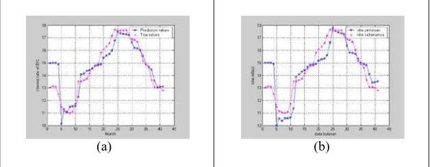
6. FORECASTING INTEREST RATE OF BANK INDONESIA CERTIFICATE USING FUZZY MODEL

In this section, singular value decomposition method is applied to forecast interest rate of Bank Indonesia Certificate (BIC) based on time series data. First, the method of sensitivity input is applied to select input variables. Second, singular value decomposition method is applied to select the optimal fuzzy relations. The initial fuzzy model with 8 input variables (8), 7), …, x(k-1)) from data of interest rate of BIC will be considered. The universal set of 8

inputs and 1 output is [10, 40] and 7 fuzzy sets A A1, 2,...,A7 are defined on each

universal set of input and output with Gaussian membership function. Then the procedure in Section 5.1 is applied to find significant inputs. The distribution of

sensitivity of input variables Ii is shown in Figure 1(a). We choose the biggest

two sensitivity of input variables Ii and three sensitivity of input variables Ii.

Based on selecting the biggest two sensitivity of input variables and three sensitivity of input variables, the selected input variables are x(k-8), x(k-1) and x(k-8), x(k-3), x(k-1), respectively.

Then time series model constructed by two input variables x(k-8) and x(k-1) has better prediction accuracy than time series model constructed by three input variables x(k-8), x(k-3), x(k-1). So we choose x(k-8) and x(k-1) as input variables to predict value x(k). Then the method of degree of fuzzy relation is applied to yield 49 fuzzy relations showed in Table 1.

[image:9.612.107.508.107.451.2]

Table 1. Fuzzy relations for interest rate of BIC using method of degree of fuzzy relation based on time series data

Rule (x t( −8),x t(−1)) →x t( ) Rule (x t( −8),x t(−1)) →x t( ) Rule (x t( −8),x t( −1))→x t( )

1 (A1, A1) →A1 17 (A3, A3) →A2 33 (A5, A5) →A1

2 (A1, A2) →A2 18 (A3, A4) →A2 34 (A5, A6) →A2

3 (A1, A3) →A2 19 (A3, A5) →A2 35 (A5, A7) →A2 4 (A1, A4) →A3 20 (A3, A6) →A2 36 (A6, A1) →A2 5 (A1, A5) →A3 21 (A3, A7) →A2 37 (A6, A2) →A2 6 (A1, A6) →A3 22 (A4, A1) →A1 38 (A6, A3) →A2 7 (A1, A7) →A3 23 (A4, A2) →A1 39 (A6, A4) →A2

8 (A2, A1) →A1 24 (A4, A3) →A2 40 (A6, A5) →A2

9 (A2, A2) →A2 25 (A4, A4) →A2 41 (A6, A6) →A2

10 (A2, A3) →A3 26 (A4, A5) →A2 42 (A6, A7) →A2

11 (A2, A4) →A3 27 (A4, A6) →A2 43 (A7, A1) →A2 12 (A2, A5) →A3 28 (A4, A7) →A2 44 (A7, A2) →A2 13 (A2, A6) →A3 29 (A5, A1) →A1 45 (A7, A3) →A2 14 (A2, A7) →A3 30 (A5, A2) →A1 46 (A7, A4) →A2

15 (A3, A1) →A1 31 (A5, A3) →A1 47 (A7, A5) →A2

16 (A3, A2) →A2 32 (A5, A4) →A1 48 (A7, A6) →A2 49 (A7, A7) →A2

(a) (b)

Figure 1. (a) Distribution of sensitivity of input variables Ii; (b) Distribution of

singular values of firing strength matrix based on time series data of interest rate of BIC

(a) (b)

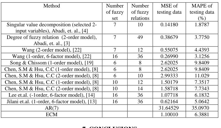
[image:9.612.149.463.549.671.2]

[image:10.612.121.493.106.321.2]

Table 2. Comparison of MSE and MAPE for forecasting interest rate of BIC using different methods

Method Number

of fuzzy set

Number of fuzzy relations

MSE of testing data

MAPE of testing data

(%) Singular value decomposition (selected

2-input variables), Abadi, et. al., [4]

7 10 0.14180 1.8787

Degree of fuzzy relation (2-order model), Abadi, et. al., [3]

7 49 0.38679 3.7750

Wang (2-order model), [22] 7 12 0.55075 4.4393 Wang (1-order, 6-factor model), [22] 16 36 0.26990 3.1256 Song & Chissom (1-order model), [19] 6 8 2.62025 9.8409 Chen, S.M & Hsu, C.C (1-order model), [8] 6 8 2.62025 9.8409 Chen, S.M & Hsu, C.C (2-order model), [8] 6 10 2.99333 11.029 Chen, S.M & Hsu, C.C (1-order model), [8] 10 12 1.50179 7.3517 Chen, S.M & Hsu, C.C (2-order model), [8] 10 14 1.58718 7.7343 Lee et.al. (-1order, 6-factor model), [14] 16 36 1.07718 6.1832 Jilani et.al. (1-order, 6-factor model), [13] 16 36 0.62164 5.0642

AR(7) 31.64529 35.0970

ECM 1.10010 6.3881

7. CONCLUSIONS

In this paper, we have presented capability of fuzzy systems to model time series data. As a universal approximator, fuzzy systems have capability to model non stationary time series. The uniqueness of fuzzy system is that the system can formulate problems based on expert knowledge or empirical data. We also presented a method to select input variables and reduce fuzzy relations of time series model based on training data. The method was used to get significant input variables and optimal number of fuzzy relations. We applied the proposed method to forecast the interest rate of BIC. The result was that forecasting interest rate of BIC using the proposed method has a higher accuracy than that using conventional time series methods.

References

[1] Abadi, A.M., Subanar, Widodo and Saleh, S., Designing fuzzy time series model and its application to forecasting inflation rate. 7Th World Congress in Probability and Statistics. Singapore: National University of Singapore, 2008. [2] Abadi, A.M., Subanar, Widodo, Saleh, S., Constructing Fuzzy Time Series Model

Using Combination of Table lookup and Singular Value Decomposition Methods and Its Applications to Forecasting Inflation Rate, Jurnal ILMU DASAR, 10(2), 190-198, 2009.

[3] Abadi, A.M., Subanar, Widodo, Saleh, S., A New Method for Generating Fuzzy Rules from Training Data and Its Applications to Forecasting Inflation Rate and Interest Rate of Bank Indonesia Certificate, Journal of Quantitative Methods, 5(2), 78-83, 2009.

[4] Abadi, A.M., Subanar, Widodo, Saleh, S., Fuzzy Model for Forecasting Interest Rate of Bank Indonesia Certificate, Proceedings of the 3rd International Conference on Quantitative Methods Used in Economics and Business, Faculty of Economics, Universitas Malahayati, Bandar Lampung, June 16-18, 2010. [5] Bollerslev, T., Generalized Autoregressive Conditional Heteroscedasticity, Journal

of Econometrics, 31, 307-327, 1986.

[6] Box, G.E.P. and Jenkins, G.M., Time Series Analysis: forecasting and Control, Holden-Day, San Francisco, 1970.

[7] Chatfield, C., The Analysis of Time Series: An Introduction, Sixth Edition, Chapman & Hall/CRC Press, Boca Raton, 2004.

234-244, 2004.

[9] Engle, R.F., Autoregressive Conditional Heteroscedasticity with Estimate of Variance of United Kingdom Inflation, Econometrica, 50, 987-1008, 1982. [10] Golub, G.H., Klema, V., Stewart, G.W., Rank Degeneracy and Least Squares

Problems, Technical Report TR-456, Dept. of Computer Science, University of Maryland, College Park, 1976.

[11] Huarng, K., Effective Lengths of Intervals to Improve Forecasting in Fuzzy Time Series, Fuzzy Sets and Systems 123, 387-394, 2001.

[12] Hwang, J.R., Chen, S.M., Lee, C.H., Handling Forecasting Problems Using Fuzzy Time Series, Fuzzy Sets and Systems 100, 217-228, 1998.

[13] Jilani, T.A, Burney, S.M.A., Ardil, C., Multivariate High Order Fuzzy Time Series Forecasting for Car Road Accidents. International Journal

of Computational Intelligence, 4(1), 15-20, 2007.

[14] Lee, L.W., Wang, L.H., Chen, S.M., Leu, Y.H., Handling Forecasting Problems Based on Two-factors High Order Fuzzy Time Series, IEEE Transactions on Fuzzy Systems, 14(3), 468 – 477, 2006.

[15] Makridakis, S., Wheelwright, S.C., Hyndman, R.J., Forecasting: Methods and Applications, Chichester: Wesley, New York, 1998.

[16] Popoola, A.O., Fuzzy-wavelet Method for Time Series Analysis, Dissertation, Department of Computing, School of Electronics and Physical Sciences, University of Surrey, Guildford, UK, 2007.

[17] Saez, D. and Cipriano, A., A New Method For Structure Identification Of Fuzzy Models And Its Application To A Combined Cycle Power Plant, Engineering Intelligent Systems, 2, 101-107, 2001.

[18] Sah, M. and Degtiarev, K.Y., Forecasting Enrollments Model Based on First-Order Fuzzy Time Series, Transaction on Engineering Computing and Technology IV, 2004.

[19] Song, Q. and Chissom, B.S., Forecasting Enrollments with Fuzzy Time series Part I, Fuzzy Sets and Systems 54, 1-9, 1993.

[20] Tseng, F-M, Tseng, G-H, Yu, H-C, Yuan, B.J.C., Fuzzy ARIMA Model for Forecasting The Foreign Exchange Market, Fuzzy Sets and Systems, 118, 9-19, 2001.

[21] Wang L.X., Adaptive Fuzzy Systems and Control: Design and Stability Analysis, Prentice-Hall, Inc., New Jersey, 1994.

[22] Wang L.X., A Course in Fuzzy Systems and Control, Prentice-Hall, Inc., New Jersey, 1997.

[23] Wang, L.X., The WM Method Completed: A Flexible System Approach to Data Mining, IEEE Transactions on Fuzzy Systems, 11(6), 768-782, 2003.

[24] Yen, J., Wang, L., Gillespie, C.W., Improving the Interpretability of TSK Fuzzy Models by Combining Global Learning and Local Learning, IEEE Transactions on Fuzzy Systems, 6(4), 530-537, 1998.

[25] Zadeh, L.A., Soft Computing and Fuzzy Logic, IEEE Software, 11(6), 48-56, 1994. [26] Zhang, B-L, Coggins, R., Jabri, M.A., Dersch, D., Flower, B., Multiresolution

Forecasting for Future Trading Using Wavelet Decomposition, IEEE Transactions on Neural Networks, 12(4), 765-775, 2001.

[27] Zhang, G.P., and Qi, M., Neural Network Forecasting for Seasonal and Trend Time Series, European Journal of Operation Research, 160(2), 501-514, 2005. [28] Zimmermann, H.J., Fuzzy Sets Theory and Its Applications, Kluwer Academic

Publisher, London, 1991.

SUBANAR: Department of Mathematics, Faculty of Mathematics and Natural

Sciences, Gadjah Mada University, Indonesia E-ma

AGUS MAMAN ABADI: Department of Mathematics Education, Faculty of Mathematics and Natural Sciences, Yogyakarta State University, Indonesia