Full Terms & Conditions of access and use can be found at
http://www.tandfonline.com/action/journalInformation?journalCode=ubes20
Download by: [Universitas Maritim Raja Ali Haji] Date: 12 January 2016, At: 23:07
Journal of Business & Economic Statistics
ISSN: 0735-0015 (Print) 1537-2707 (Online) Journal homepage: http://www.tandfonline.com/loi/ubes20
Peer and Selection Effects on Youth Smoking in
California
Brian V Krauth
To cite this article: Brian V Krauth (2007) Peer and Selection Effects on Youth Smoking in California, Journal of Business & Economic Statistics, 25:3, 288-298, DOI: 10.1198/073500106000000396
To link to this article: http://dx.doi.org/10.1198/073500106000000396
Published online: 01 Jan 2012.
Submit your article to this journal
Article views: 110
View related articles
Peer and Selection Effects on Youth
Smoking in California
Brian V. K
RAUTHSimon Fraser University, Burnaby, BC V5A 1S6, Canada (bkrauth@sfu.ca)
Previous research has found that youth smoking choices are strongly influenced by peer smoking. How-ever, these studies often fail to account for simultaneity and nonrandom peer selection. This article de-scribes an equilibrium model of peer effects that incorporates both of these features, and estimates its parameters using data on California teenagers. Identification is aided by using the influence of observable variables on group selection as a proxy for the influence of unobservables. I find that the effect of peer smoking on the decision to smoke is much weaker than found in previous studies.
KEY WORDS: Binary games; Peer effects; Simulation-based estimation; Social interactions.
1. INTRODUCTION
Youth smoking is a major public health concern in much of the world. The World Health Organization (Mackay and Eriksen 2002, p. 36) estimates that 4.2 million individuals die every year from smoking-related conditions. As a result, gov-ernments often spend large sums on programs to reduce tobacco use. Because tobacco is highly addictive and most smokers be-gin when they are teenagers (Mackay and Eriksen 2002, p. 28), tobacco control efforts often focus on discouraging young peo-ple from starting to smoke. Many of these efforts aim to alter the social context of youth smoking, due to a consensus among pol-icymakers and researchers (Tyas and Pederson 1998; Mackay and Eriksen 2002) that a young person’s decision to smoke is highly influenced by the behavior and attitudes of his or her peers. From an economic standpoint, peer effects are of interest because they imply an externality that may, in principle, lead to suboptimal outcomes even among rational individuals. As a re-sult, the case for increased government intervention in tobacco markets may be strengthened by evidence of strong peer effects. In spite of the apparent consensus among researchers and pol-icymakers, the influence of peers in youth smoking is far from well established. Many empirical studies in the literature fail to account for both simultaneity and nonrandom peer selection, either of which may lead a researcher to dramatically overesti-mate the strength of peer influence (Manski 1993). More recent studies that attempt to account for Manski’s critique have found mixed results.
This article uses data from the 1994–2002 California Youth Tobacco Survey (CYTS) to estimate the strength of close-friend influence on smoking among young people. These peer effects are estimated using an equilibrium discrete choice model de-veloped in Krauth (2006) and previously applied to Canadian youth smoking data in Krauth (2005). The structural model explicitly allows for both simultaneity and nonrandom peer selection, thereby addressing key elements of Manski’s cri-tique. The article provides three key advances from the work in Krauth (2005). First, I control for a more extensive set of individual level covariates commonly found to have strong ex-planatory power for youth smoking, including race/ethnicity; disposable income; and more detailed information on smoking behavior of parents, teachers, and older siblings. Second, I de-velop and implement an asymptotically valid test for the null hypothesis of no peer effects. Such a test was unavailable in
previous work, as the usualtstatistic is not asymptotically nor-mal under the null. Third, the model is estimated under a wide variety of alternative specifications and under alternative equi-librium selection rules, providing detailed information on the robustness of the baseline results.
The general finding of this article is that close-friend effects are nonzero but substantially weaker than is commonly found in the literature. Results for the baseline structural model imply that a representative individual’s probability of self-identified current smoking increases by only one percentage point (from an initial probability of 13.2%) in response to one of four close friends becoming a smoker. While the baseline structural model is estimated under the strong assumption that the within-group correlation in unobservable characteristics is equal to the correlation in observable characteristics, an upper bound on peer effects can also be estimated under the very conserv-ative restriction that the within-group correlation in unobserved characteristics is nonnegative (i.e., a young person is at least as similar to his or her close friends as would be the case un-der random assignment). In that case, I find that the representa-tive individual’s probability of smoking rises by no more than 7.9 percentage points in response to one close friend becoming a smoker. Both the baseline estimate and the upper bound are well below nearly all reduced-form estimates found in the lit-erature, as well as reduced-form estimates based on the CYTS data. The peer effect estimates in this article are also somewhat lower than the corresponding estimates in Krauth (2005), possi-bly because of the richer set of covariates included in this study.
1.1 Related Literature
An extensive literature in health economics and public health addresses the determinants of tobacco use. Researchers have paid particular attention to youth smoking, as the strongest pre-dictor of smoking among adults is smoking as a young per-son (Gruber and Zinman 2001). Variables that consistently have predictive power for youth smoking include parental or sib-ling smoking, performance in school, race/ethnicity, dispos-able income, and prices, as well as peer smoking (Tyas and
© 2007 American Statistical Association Journal of Business & Economic Statistics July 2007, Vol. 25, No. 3 DOI 10.1198/073500106000000396
288
Pederson 1998). However, the finding of a close statistical asso-ciation between peer smoking and a respondent’s own smoking does not necessarily imply a causal relationship. Indeed, selec-tion (the tendency of young people to form peer groups with others who have similar preferences and backgrounds) and si-multaneity (that a young person’s behavior both influences and is influenced by the behavior of his or her peers) imply that reduced form regression coefficients may dramatically over-state the strength of any causal relationship. Although this is-sue was known well before Manski’s influential 1993 article, it is only recently that empirical studies of youth smoking that at-tempt to account for selection and simultaneity have appeared. In addition to the structural approach pursued in this article, two alternative approaches appear regularly in the youth smoking literature. One method is to use group characteristics as instru-mental variables for group behavior (Norton, Lindrooth, and Ennett 1998; Gaviria and Raphael 2001; Powell, Tauras, and Ross 2005). A more indirect method (Engels, Knibbe, Drop, and de Haan 1997; Wang, Eddy, and Fitzhugh 2000) is to ask whether smoking tends to precede or follow membership in a peer group of smokers. Krauth (2005) provided a discussion of the advantages and disadvantages of these three approaches.
The structural model and estimation method were developed in Krauth (2006). That article also provided a brief empirical application to 1989 U.S. youth smoking data as illustration, though the absence of state identifiers (and thus prices) from the dataset leaves the results subject to substantial omitted-variables bias. Krauth (2005) provided a more detailed em-pirical application using 1994 Canadian data with province identifiers. Other articles estimating equilibrium models of youth smoking include Nakajima (2004) and Kooreman and Soetevent (2006). Both of these articles differ from the current article and from Krauth (2005) in that they estimate classroom level peer effects rather than close-friend effects and they use only aggregate level fixed effects (at the school level for Koore-man and Soetevent, and the county level for Nakajima) to ac-count for nonrandom peer selection.
2. DATA
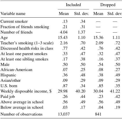
The CYTS is an annual cross-sectional household-based sur-vey of California youth aged 12 to 17 (California Department of Health Services 2003). This study uses results from 1994 through 2002 and restricts attention to respondents from age 14 through 17. The original dataset contains 13,878 observations in this age range, of which 13,037 have sufficient information for use in estimating the structural model. Summary statistics, after the data cleaning and imputations outlined in the following discussion, are reported in Table 1.
2.1 Variable Construction
For each observation, there are two endogenous variables: a binary variable indicating the current smoking status of the respondent and a variable indicating the fraction of the respon-dent’s closest same-sex friends that smoke. The respondent is defined as a current smoker if he or she reports having smoked at least one cigarette in the previous 30 days. This measure of smoking prevalence is standard in the literature. The peer smok-ing rate is defined as the respondent’s estimate of the fraction
Table 1. Summary statistics for 1994–2002 CYTS data Included Dropped Variable name Mean Std. dev. Mean Std. dev. Current smoker .13 .34 — — Fraction of friends smoking .21 .31 — — Number of friends 4.04 1.37 — — Age 15.43 1.10 15.36 1.11 Teacher’s smoking (1–3 scale) 2.16 .70 2.09 .72 Discussed health risks in class .77 .42 .76 .42 At least one parent smokes .33 .47 .32 .47 At least one sibling smokes .17 .38 .16 .37 Male .50 .50 .54 .50 African-American .07 .25 .08 .27 Hispanic .36 .48 .38 .49 Asian/other .09 .29 .09 .29 U.S. born .87 .34 .85 .35 Weekly disposable income, $ 29.98 40.20 30.04 41.22 Paid job .26 .44 .23 .42 Above average in school .56 .49 .56 .49 Below average in school .03 .17 .04 .19 Number of observations 13,037 841
NOTE: Columns labeled “Included” describe data included in the estimation; columns labeled “Dropped” describe data dropped because of missing data on endogenous variables (current smoking and/or friend smoking).
of his or her same-sex best friends that smoke. The construc-tion of this variable varies somewhat in different years of the CYTS. In the 1994–1999 surveys, the respondent is asked how many best friends of each sex he or she has, and then how many of these friends smoke. The number of best friends of each sex can vary from 0 to 70. In the 2000–2002 surveys, the respon-dent is not asked the number of best friends, but is simply asked how many of his or her four best friends of each sex smoke. To keep the computational time for the structural estimator reason-able, it is necessary to place a cap on the number of friends. Any respondent who reports more than six close friends is re-coded as having exactly six friends, and the fraction of friends who smoke is rounded to the nearest sixth. For example, if a respondent reports ten close friends, seven of whom smoke, he is coded as having six close friends, four (6×7/10=4.2≈4) of whom smoke. Those respondents who did not report their own smoking behavior (76 observations) or that of their close friends (92 observations), or who reported having zero best friends (673 observations) were dropped from the sample. For comparison, summary statistics for the observations that were dropped from the sample are reported in Table 1. As the table shows, those respondents who were dropped from the sample are similar in observable characteristics to those who are in-cluded.
In addition to these variables, the CYTS includes information on demographics, family, workplace and school environment, attitudes, and other risky behavior. The explanatory variables included in the model are year; age; ethnicity; whether parents, teachers, or older siblings smoke; immigrant status; weekly disposable income; employment; performance in school; and classroom exposure to information about the risks of smoking. Disposable income is top coded at $200 per week, and missing values for disposable income are replaced with the sample me-dian of $15. Missing values for the other explanatory variables are replaced by the sample mean for that variable. In all, 459 of
the 13,037 observations feature one or more imputations. As re-ported in Table 2, reduced-form coefficient estimates are nearly identical when the model is reestimated either with observa-tions with missing variables dropped or with an additional indi-cator variable for whether an observation had values imputed.
Note that the CYTS is based on a stratified random sample of individual youth, rather than on a group-based sample. This has two implications that complicate estimation of the model. First, only the characteristics of the respondent and not those of his or her peers are observed. With a group-based sample (e.g., a survey of all students in a random sample of California secondary schools), the within-group correlation in observable characteristics could be estimated directly. With an individual-based sample like the CYTS, this correlation is identified through a less direct channel: All else being equal, a higher within-group correlation in observable characteristics implies a stronger relationship between the observable characteristics of the respondent and the behavior of his or her peers, after controlling for the respondent’s own behavior. Krauth (2006) provided a detailed discussion of identification in the model presented here. The second issue created by the use of an individual-based sample is that there is no assurance that a respondent’s own smoking and that of his or her peers are reported consistently. In particular, the average self-reported smoking rate of CYTS respondents (13.2%) is substantially lower than the rate of smoking they report for their friends (21.3%). This is most likely due to a combination of smokers falsely self-identifying as nonsmokers and respondents overes-timating the smoking rate of peers. This inconsistent reporting must be accounted for in the structural econometric model.
2.2 Trends in Youth Smoking and Tobacco Control in California
Before describing the econometric model, it is useful to con-sider the basic trends in California relevant to youth smoking. Figure 1 shows the rate of self-reported current smoking among age 14–17 CYTS respondents by year, as well as the rate of self-reported current smoking among U.S. high school students as
Figure 1. Rates of current smoking among young people in Cali-fornia and entire United States, 1993–2002. CaliCali-fornia smoking rates are based on author’s calculations using CYTS; national smoking rates are based on CDC estimates.
calculated by the Centers for Disease Control and Prevention (CDC 2002a, b, 2003). Throughout the sample period, Califor-nia youth are approximately half as likely to smoke as youth in the United States as a whole. Clearly, there are important state-specific factors operating in California to make cigarette smok-ing relatively less attractive to youth. Any extrapolation of this study’s findings to the rest of the United States must recognize that, while it can be thought of as somewhat representative due to its cultural and economic diversity and its large urban, sub-urban, and rural populations, California is in other ways very different from the rest of the United States.
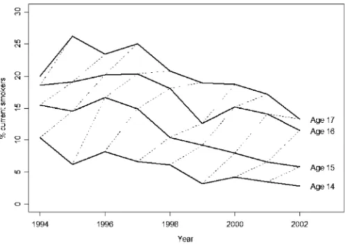
By some measures, California’s tobacco control policy was fairly typical over the sample period. California’s excise tax rates—tied for 15th in 1994, 18th in 2002 (Orzechowski and Walker 2002)—and level of per-capita expenditure on tobacco control—19th in 2002 (CDC 2002a)—are above the median among U.S. states, though far from the highest. However, the sample period saw two major changes in California’s tobacco control policy. The first was the passage of legislation that required almost all workplaces, including restaurants, to be smoke free beginning in January 1995, and bars to be smoke free beginning in January 1998. California was one of the ear-liest adopters of the workplace smoking ban, a tobacco control strategy that has since been adopted by many other jurisdictions both inside and outside the United States. The second major policy change was the January 1999 increase in state excise taxes from 37 cents to 87 cents per pack, as a result of the passage of the voter initiative known as Proposition 10. This was California’s only change in cigarette excise taxes during the sample period. Figure 1 shows a sizable decline in youth smoking from 1997 to 1999, possibly related to these policy changes, but possibly also related to unmeasured trends in so-cial norms. Figure 2 breaks down these aggregate trends by age. Each solid line in the figure represents the time path of smoking rates for a particular age group, while each dashed line follows the time path of smoking rates within a particular birth cohort. As the figure shows, the smoking rate of an individual cohort usually increases over time, even as aggregate youth smoking is falling. The overall downward trend in smoking rates applies to all age groups.
Figure 2. Rates of current smoking among young people in CYTS by year and age. Dashed lines connect members of the same birth co-hort.
3. METHODOLOGY
The econometric model is similar in spirit to the standard model of discrete choice with social interaction effects de-scribed in Brock and Durlauf (2001). Krauth (2006) dede-scribed both the model and the estimation method in greater detail.
3.1 Model
Each individual is a member of exactly one peer group. Within each group g∈Z+, individuals are indexed by i∈ {1,2, . . . , ng}, so that the pairi, g identifies an individual. An individual can choose either to be a current smoker (si,g=1) or not (si,g=0). Lettingsg≡(s1,g, . . . , sn
g,g), we can see that an
individual’s utility functionui,g(si,g;sg)satisfies
ui,g(1;sg)−ui,g(0;sg)=α+βxi,g+λzg+γs¯i,g+ǫi,g, (1)
wherexi,g is akx-length vector of individual level exogenous variables, zg is a kz-length vector of group level exogenous variables, ands¯i,g is the fraction of the other group members that smoke (i.e., s¯i,g≡ ng1−1j=isj,g). This model thus in-corporates an endogenous peer effect (γs¯i,g) into an otherwise standard discrete choice model of smoking. As in the standard model, an individual prefers to smoke if and only if his or her incremental utility from doing so is positive:
(si,g=1) ⇔ (α+βxi,g+λzg+γs¯i,g+ǫi,g≥0). (2) Note that endogenously determined behavior appears on both sides of this expression. Also note that the model does not in-clude contextual effects, in which the characteristics (as op-posed to smoking behavior) of one’s peers have a direct effect on the relative utility of smoking. Since Manski (1993) pointed out the difficulties in doing so, empirical researchers rarely at-tempt to simultaneously estimate endogenous effects and con-textual effects. It is more common (e.g., Hoxby 2000; Gaviria and Raphael 2001; Sacerdote 2001) to simply ignore one or the other and note that the estimated endogenous (contextual) effect could be reinterpreted as contextual (endogenous). That caveat applies to this study as well.
One consequence of the endogeneity of peer smoking is that an equilibrium outcome must be explicitly defined. In all of the empirical analysis in this article, the observed choices of individuals are assumed to correspond to a Nash equilibrium, with a selection rule to be applied when there are multiple Nash equilibria. For the baseline results, the endogenous variables are assumed to take on the values associated with the lowest-activity Nash equilibrium for the given exogenous variables. The lowest-activity Nash equilibrium is defined as the Nash equilibrium with the fewest smokers:
sg=mins∈ {0,1}ng:(si=1)⇔ui,g(1;s) > ui,g(0;s).
(3)
Because this is a game with strategic complementarities (also known as a “supermodular” game), the lowest-activity Nash equilibrium always exists and is unique (Milgrom and Roberts 1990, thms. 5 and 6). Krauth (2006) argued that the static lowest-activity Nash equilibrium provides a reasonable approximation to the outcome of a more realistically specified dynamic interaction process. To check the robustness of the
baseline results to this equilibrium selection rule, the model will also be estimated under the assumption that the highest-activity Nash equilibrium is selected, and under the assumption that groups randomize among all pure strategy Nash equilibria. A second consequence of the endogeneity of peer choice is that the model must address inconsistent reporting of smok-ing behavior. The substantial difference between self-reported and peer-reported smoking rates described in Section 2.1 could not be an equilibrium outcome unless a distinction is made be-tween actual and reported behavior. Let ri,g equal 1 if person i, g self-identifies as a smoker and 0 otherwise. The relation-ship between actual and self-reported behavior is assumed to be
ri,g=
si,g with probabilitypr 0 with probability 1−pr,
(4)
where pr is a parameter to be estimated. In other words, an exogenous fraction of smokers falsely self-identify as non-smokers, and everyone else reports truthfully. Audit studies (e.g., Wagenknecht, Burke, Perkins, Haley, and Friedman 1992) that compare self-reports to biochemical indicators from breath and saliva tests indicate such underreporting is common. Krauth (2005) used Monte Carlo simulations to consider alter-native models of inconsistent reporting, including both random and biased (i.e., smokers are more likely to overestimate the smoking of peers than are nonsmokers) overreporting of peer smoking. The results there imply that a finding of weak peer effects is robust to these alternatives.
The third consequence of the endogeneity of peer smoking is that it is necessary to model the unobserved preferences of peers. In this model, the joint distribution of the individual level exogenous variables is assumed to be multivariate normal and independent across groups but correlated among members of a given peer group. Allowing for a within-group correlation in preferences is critical, because failure to account for correlated preferences can lead researchers to mistake peer similarity for peer influence. For a group of sizeng=3, the distribution takes the form:
with the distribution being defined analogously for other values ofng.
Although the model is sufficiently nonlinear to be formally identified without further restrictions, additional restrictions will be placed on the within-group correlation in unobservables. Without these restrictions, identification may rely too heavily on the arbitrary assumption of normality rather than on more
substantive assumptions. For the baseline results, it is assumed that the correlation in unobservable characteristics is equal to the correlation in observables:
ρǫ=ρx. (6)
The idea of using the degree of selection on observables as a reasonable guess at the degree of selection on unobservables was proposed by Altonji, Elder, and Taber (2005) to correct for selection effects in measuring the effect of attending a Catholic school. The intuition supporting the equal-correlation assump-tion is that equality in the two correlaassump-tions will hold in expec-tation if the observables are a random subset of a large set of relevant variables. Alternatively, if variables that are more likely to be observed in survey data (e.g., race, sex, age) are also more easily observed by potential friends, then ρx will provide an upper bound onρǫ. Although the baseline equal-correlation as-sumption provides a useful and plausible starting point, I also estimate the model under alternative restrictions onρǫ.
3.2 Estimation
The model is estimated by simulated maximum likelihood (SML). Krauth (2006) described the estimator and its properties in detail, provided a discussion of identification, and reported the outcome of various Monte Carlo experiments. The para-meter vector to be estimated is θ ≡(γ , α, β, λ, pr, μ, σ, ρx,
for some small δ >0 and some largeM. The restrictions on ρxandρǫare needed to guarantee that the within-group covari-ance matrix of characteristics is positive definite. The likelihood function for the dataℓN(θ )is defined as
where N is the number of observations in the data and the gth observation in the dataset is taken to identify person 1 of group g. The baseline SML estimator θˆN imposes the equal-correlation restriction:
where ℓˆN(θ ) is a simulation-based estimate of the true log-likelihood functionℓN(θ ). In addition, the model will be esti-mated for specific values ofρǫ. Let the functionθˆN: [0,1)→
By the theorem of the maximum, continuity ofℓˆNimplies con-tinuity ofθˆN(ρ)so this function can be approximated by calcu-lating at each value ofρon a sufficiently fine grid. The function
ˆ
θN(ρ)can be used to place consistent bounds on parameter val-ues for any interval restriction onρǫ.
In addition to the structural model estimates, Section 4 also reports results for a “naive” or reduced-form probit model in which peer behavior is exogenous. This reduced-form estimator corresponds to the standard approach in much of the literature. The model takes the form:
Pr(r1,g=1|x1,g, zg,s¯1,g)
=pr(α˜+ ˜βx1,g+ ˜λzg+ ˜γs¯1,g), (11)
whereis the cumulative distribution function (cdf ) for the standard normal distribution. The model is estimated by max-imum likelihood both under the conventional assumption of truthful reporting (pr =1) and under the model of underre-porting described in Section 3.1.
Because the two reduced-form models and the structural models do not have identical functional forms, coefficient es-timates are not directly comparable unless converted into mar-ginal effects for a representative individual. Letr¯ be the rate of self-reported smoking in the population and let the repre-sentative individual be a hypothetical person whose observable characteristics imply Pr(r1,g =1|x1,g, zg,s¯1,g)= ¯r. For this representative individual, equation (11) implies that the mar-ginal effect ofx1,g on the probability of being a self-reported smoker is given by prφ (−1(r/p¯ r))β˜. The tables of results in Section 4 report coefficient estimates as well as the factor prφ (−1(r/p¯ r))by which they can be multiplied to generate marginal effects.
3.3 Inference
The model is estimated under the maintained hypothesis of nonnegative peer effects, that is, that γ ≥0. If the true value ofγ is strictly positive, inference in this model is stan-dard: Parameter estimates are asymptotically normal with a covariance matrix that can be consistently estimated by con-ventional methods. However, inference is nonstandard un-der the boundary case of no peer effects (γ =0). In that case, the bootstrap standard errors reported in Section 4 are inconsistent (Andrews 2000), and the parameter estimates and associated test statistics have non-Gaussian asymptotic distributions (Andrews 2001). As a result, previous work (Krauth 2005, 2006) using this model and estimation method did not provide a test for the null hypothesis of no peer effects. This section describes a simple test that will be implemented in Section 4.
Let the null hypothesis beH0:γ =0 and the alternative hy-pothesis beH1:γ >0. Let the likelihood ratio (LR) test
statis-tic be given by
Under the null, Theorem 4 in Andrews (2001; see also sec. 5.6) implies that the test statisticLRN converges in distribution to a nonnegative random variable with cdf:
F (x)=.5+
2(1)distribution. The results
re-ported in Section 4 include both theLRN statistic and its as-ymptoticpvalue.
4. RESULTS
4.1 Naive Model Estimates
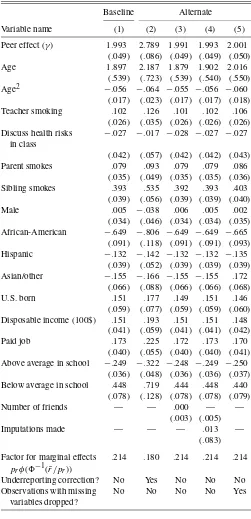
Table 2 reports coefficient estimates for the reduced-form model. In addition to the variables reported in the table, year ef-fects are included in the regressions to control for any aggregate shocks such as the policy changes described in Section 2.2. The main specification is estimated both without the underreporting correction (1) and with the correction (2). Specifications (3)–(5) provide robustness checks on the main results. In addition to co-efficient and standard error estimates, each column in Table 2 also reports a “Factor for marginal effects,” described in the last paragraph of Section 3.2, which can be multiplied by each
coef-Table 2. Regression results for reduced form (naive) model Baseline Alternate Variable name (1) (2) (3) (4) (5) Peer effect (γ) 1.993 2.789 1.991 1.993 2.001
(.049) (.086) (.049) (.049) (.050) Age 1.897 2.187 1.879 1.902 2.016
(.539) (.723) (.539) (.540) (.550) Age2 −.056 −.064 −.055 −.056 −.060
(.017) (.023) (.017) (.017) (.018) Teacher smoking .102 .126 .101 .102 .106
(.026) (.035) (.026) (.026) (.026) Discuss health risks −.027 −.017 −.028 −.027 −.027
in class
(.042) (.057) (.042) (.042) (.043) Parent smokes .079 .093 .079 .079 .086
(.035) (.049) (.035) (.035) (.036) Sibling smokes .393 .535 .392 .393 .403
(.039) (.056) (.039) (.039) (.040) Male .005 −.038 .006 .005 .002
(.034) (.046) (.034) (.034) (.035) African-American −.649 −.806 −.649 −.649 −.665
(.091) (.118) (.091) (.091) (.093) Hispanic −.132 −.142 −.132 −.132 −.135
(.039) (.052) (.039) (.039) (.039) Asian/other −.155 −.166 −.155 −.155 .172
(.066) (.088) (.066) (.066) (.068) U.S. born .151 .177 .149 .151 .146
(.059) (.077) (.059) (.059) (.060) Disposable income (100$) .151 .193 .151 .151 .148
(.041) (.059) (.041) (.041) (.042) Paid job .173 .225 .172 .173 .170
(.040) (.055) (.040) (.040) (.041) Above average in school −.249 −.322 −.248 −.249 −.250
(.036) (.048) (.036) (.036) (.037) Below average in school .448 .719 .444 .448 .440
(.078) (.128) (.078) (.078) (.079) Number of friends — — .000 — —
(.003) (.005) Imputations made — — — .013 —
(.083) Factor for marginal effects .214 .180 .214 .214 .214
prφ(−1(r/p¯ r))
Underreporting correction? No Yes No No No Observations with missing No No No No Yes
variables dropped?
ficient estimate to convert the coefficient into an estimated mar-ginal effect. This conversion is needed to make comparisons across models, as the raw coefficients of the underreporting-corrected and -ununderreporting-corrected models are not directly comparable. Standard errors are estimated using the inverse Hessian of the log-likelihood function.
The results are roughly consistent with the previous literature on youth smoking. Young people are more likely to smoke if they are older; if they are exposed to parents, teachers, and sib-lings who smoke; if they have more disposable income and/or a job; and if they are doing poorly in school. They are less likely to smoke if they are doing well in school. In addition, there are substantial differences across ethnic and cultural groups in youth smoking rates, even after controlling for a number of variables that vary across those groups. In California dur-ing this period, African-American, Hispanic, and Asian/other young people had a particularly low probability of smoking, as did young people born outside of the United States.
Taken at face value, the results in Table 2 also suggest that peers are quite influential. The peer effect coefficient is statisti-cally significant at all conventional levels, and is quite large. The marginal effect of peer smoking ranges from .43 to .50 across the two main specifications. Section 4.3’s comparison of the results in this article with the literature shows that the re-sults in Table 2 are similar to those found by other researchers using reduced-form models.
The remaining specifications in Table 2 provide robustness checks. Specification (3) uses the original unadjusted data for number of friends and fraction of friends smoking and includes the number of friends as an exogenous explanatory variable. It is provided as a check that truncating the number of friends as described in Section 2.1 does not have a dramatic effect on at least a simple model of the data and that the number of friends is not an important explanatory variable. Specifications (4) and (5) provide robustness checks on the handling of observations with missing data: (4) is estimated with an indicator variable for any observation in which variables have been imputed, whereas (5) is estimated after dropping the 459 observations with miss-ing data. For all three alternative specifications, coefficient esti-mates are similar to those of the baseline reduced-form specifi-cation.
4.2 Structural Model Estimates
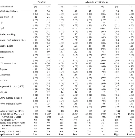
Table 3 reports point estimates for the structural model with the baseline assumption of equal correlation in observables and unobservables. In addition to the individual level variables re-ported in the table, year effects are included and are treated as aggregate variables (zg in the model). The underreporting cor-rection is used, and standard errors are estimated using the sim-ple bootstrap with 100 replications. Column (1) shows the main specification, and the remaining columns show several alterna-tive specifications.
The results in Table 3 imply much weaker peer influence than is implied by the reduced-form estimates in Table 2. The estimated marginal effect of peer smoking in specification (1) is less than 10% as large as the corresponding marginal effect from Table 2. To understand why the estimated peer effect falls so much from the reduced-form probit model to the structural
Table 3. Regression results for structural model
Baseline Alternate specifications
Variable name (1) (2) (3) (4) (5) (6) (7) (8) Selection effect (ρ) .55 .54 .50 .47 .47 .52 .58 .52
(.06) (.06) (.07) (.07) (.08) (.05) (.04) (.08) Peer effect (γ) .22 .26 .33 .38 .38 .32 .14 .32
(.18) (.18) (.20) (.21) (.22) (.16) (.11) (.26) Age .71 .75 .65 .65 .67 .88 .77 .65
(.44) (.38) (.38) (.37) (.36) (.57) (.51) (.63) Age2 −.01 −.02 −.02 −.02 −.02 −.02 −.02 −.01
(.01) (.01) (.01) (.01) (.01) (.02) (.08) (.02) Teacher smoking .24 .24 .25 .15 .16 .24 .24 .24
(.02) (.02) (.03) (.01) (.01) (.02) (.02) (.03) Discuss health risks in class −.08 −.08 −.07 −.07 −.07 −.09 −.08 −.08
(.03) (.04) (.03) (.02) (.02) (.03) (.04) (.04) Parent smokes .28 .27 .28 .28 .29 .28 .28 .28
(.03) (.04) (.03) (.03) (.04) (.03) (.04) (.03) Sibling smokes .59 .59 .61 .62 .62 .61 .58 .61
(.05) (.05) (.05) (.05) (.05) (.04) (.06) (.05) Male .07 .06 .06 .06 .06 .07 .07 .07
(.03) (.03) (.03) (.03) (.02) (.03) (.03) (.03) African-American −.54 −.56 −.60 −.61 −.62 −.60 −.54 −.58
(.08) (.07) (.09) (.08) (.09) (.08) (.09) (.10) Hispanic −.09 −.10 −.11 −.11 −.12 −.10 −.09 −.11
(.04) (.04) (.04) (.04) (.04) (.03) (.03) (.04) Asian/other −.12 −.12 −.13 −.14 −.13 −.14 −.11 −.13
(.06) (.05) (.06) (.06) (.05) (.06) (.05) (.06) U.S. born .24 .25 .24 .25 .24 .26 .23 .24
(.05) (.05) (.06) (.05) (.05) (.05) (.05) (.06) Disposable income (100$) .34 .35 .37 .37 .36 .35 .47 .35
(.04) (.04) (.04) (.04) (.04) (.03) (.14) (.04) Paid job .12 .12 .14 .14 .15 .12 .11 .12
(.04) (.03) (.04) (.04) (.04) (.04) (.04) (.04) Above average in school −.51 −.51 −.52 −.53 −.53 −.54 −.51 −.53
(.04) (.04) (.04) (.04) (.04) (.03) (.04) (.04) Below average in school .77 .75 .81 .81 .80 .80 .74 .79
(.10) (.10) (.10) (.11) (.10) (.09) (.10) (.10) Factor for marginal effects .180 .180 .180 .180 .180 .180 .180 .180 LR statistic forH0:γ=0 5.238 8.487 10.011 66.577 55.230 13.923 12.479 13.392
Asymptoticpvalue .011 .002 .001 .000 .000 .000 .000 .000 Year-specificpr? No Yes No No No No No No
Treated as aggregate: Age? No No Yes Yes Yes No No No School environment? No No No Yes Yes No No No
Sex? No No No No Yes No No No
Dropped if no friends? Yes Yes Yes Yes Yes No Yes Yes Equilibrium selected Low Low Low Low Low Low High Random
model, note that the estimated ρx is quite high. This means that in the data a respondent’s characteristics are highly cor-related with the smoking behavior of his or her peers, even af-ter controlling for the respondent’s own behavior. In the model, this feature of the data implies high ρx, and with the equal-correlation assumption, it also implies highρǫ. Once the cor-relation in characteristics across peers is accounted for, there is very little residual correlation in behavior. As a result, the es-timated peer effect (γ) is much lower for the structural model than for the reduced-form model.
Table 3 also reports the LR test statistic defined in equa-tion (12) for the null hypothesis H0:γ =0 against the
alter-nativeH1:γ >0. According to the LR test statistic, one can reject the null hypothesis of no peer effect at the 5% asymptotic significance level, though not quite at the 1% level. At the same time, thet statistic forγ is below the usual asymptotic criti-cal values, implying that one cannot reject the nullγ=δfor a small but strictly positive value ofδ.
The remaining columns in Table 3 provide some basic ro-bustness checks. Specification (2) allows for the reporting rate pr to vary from year to year and provides results nearly identical to those for the baseline specification. Specifica-tions (3)–(5) are identical to specification (1), except that some additional variables are treated as aggregate. Recall thatρx is
the within-group correlation in individual level variables, so counting a group level variable—which is, by definition, per-fectly correlated among group members—as an individual level variable will tend to raise estimates ofρxand lower estimates ofγ. To provide a robustness check on the baseline specifica-tion, the model is estimated treating age, school characteristics (Teacher smoking and Discuss health risks in class), and/or sex as aggregate variables. As the table shows, treating age and/or school characteristics as aggregate variables does lead to a mod-erately lower estimate ofρx and a moderately higher estimate ofγ. Specification (6) is identical to specification (1), but in-cludes in the sample the 673 respondents who self-identified as having no close same-sex friends. The peer smoking variable
¯
si,gis coded as 0 for those respondents. Specifications (7) and (8) show results from estimating the baseline model under al-ternative equilibrium selection rules. In specification (7), peer groups are assumed to always play the highest-smoking Nash equilibrium. In specification (8), peer groups are assumed to randomize among pure strategy Nash equilibria. Overall, the es-timated peer effect and selection effect varies somewhat across alternative specifications, but the range of estimates is not very wide. The estimated within-group correlation in characteristics ranges from .47 to .58, whereas the estimated marginal peer effect ranges from .03 to .07, well below the baseline reduced-form estimate of .43 to .50.
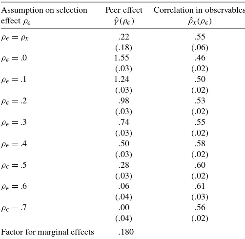
The equal-correlation assumption represents the most criti-cal potential source of misspecification in the baseline model. Though simple and plausible, this assumption is certainly open to question. To address this issue, Table 4 displays estimates of theγ (ˆ ·)andρˆx(·)functions as described in Section 3.2. Stan-dard errors are estimated by the simple bootstrap with 50 repli-cations each. Note that γ (ρˆ ǫ) is decreasing in ρǫ, whereas
ˆ
ρx(ρǫ)is increasing inρǫ. A higherρǫ means that more cor-relation in behavior can be explained by corcor-relation in prefer-ences, and there is less need to explain the data with a strong
Table 4. Estimated peer/selection effect under alternative identifying restrictions
Assumption on selection Peer effect Correlation in observables effectρǫ γˆ(ρǫ) ρˆx(ρǫ)
ρǫ=ρx .22 .55
(.18) (.06)
ρǫ=.0 1.55 .46
(.03) (.02)
ρǫ=.1 1.24 .50
(.03) (.02)
ρǫ=.2 .98 .53
(.03) (.02)
ρǫ=.3 .74 .55
(.03) (.02)
ρǫ=.4 .50 .58
(.03) (.02)
ρǫ=.5 .28 .60
(.03) (.02)
ρǫ=.6 .06 .61
(.04) (.03)
ρǫ=.7 .00 .56
(.04) (.02) Factor for marginal effects .180
peer effect. This is whyγ (ˆ ·)is decreasing inρǫ. At the same time, the correlation between the respondent’s characteristics and the behavior of peers is increasing inγ, all else equal. As
ˆ
γ (ρǫ)is decreasing inρǫ, more of the observed correlation be-tween respondent observed characteristics and peer behavior must be explained by correlation in observed characteristics. This is whyρˆx(ρǫ)is increasing inρǫ.
To interpret Table 4, note, for example, that the SML esti-mate of the peer effect under no selection effect (ρǫ=.0)is
ˆ
γ (.0)=1.55. The associated marginal effect is .28, well above the marginal effect implied by the baseline model (.04) but well below that implied by the reduced-form model (.43–.50). In other words, the structural estimates are well below the reduced-form estimates even in the absence of a selection ef-fect; the reason for this is that the simultaneity bias (present in the reduced-form model, but not in the structural model) is quite large when the peer group is small. As indicated in Sec-tion 3.2, these results can also be used to place consistent and potentially informative bounds on the peer effect under any in-terval restriction on the selection effect. For example, suppose that the correlation in unobservables is at least nonnegative (i.e., close friends are at least as similar in unobserved preferences as randomly constructed groups of individuals would be). The es-timated upper bound onγ under the restrictionρǫ ≥0 is ap-proximately 1.55. If, following the argument in Section 3.1, one takes ρx as an upper bound on ρǫ, then the estimated lower bound onγ subject to the restrictionρǫ≤.55 is approxi-mately .22. Readers with stronger or weaker prior beliefs on the value ofρǫ can use Table 4 to construct alternative bounds on the peer effect.
Figure 3 summarizes this article results graphically. The solid line is theγ (ρ)ˆ function, converted into marginal effects, and the shaded area surrounding it represents a pointwise 95% as-ymptotic confidence band. The two points on the left side of the graph represent marginal effects associated with each of the reduced-form estimates (which implicitly assume no selection
Figure 3. Estimated marginal peer effect [γprφ(−1(r/p¯ r))] for
alternative assumptions about selection effect (ρǫ). Individual points
represent point estimate from the reduced-form probit model or the baseline structural model with equal correlation assumption. The el-lipse depicts the 95% confidence region for the structural model esti-mate. The solid line is based on theγˆ(ρ) function, and the shaded area depicts the 95% pointwise confidence band.
effect). The point in the center represents the marginal effect as-sociated with the point estimate from the structural model under the equal-correlation assumption, and the ellipse surrounding it is a 95% joint asymptotic confidence region.
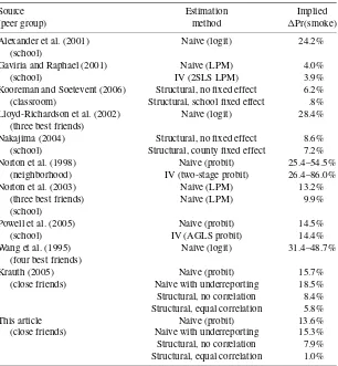
4.3 Interpretation and Comparison to Previous Findings
Having established the primary quantitative results of this ar-ticle, it remains to place them in the context of previous studies. To give the estimated coefficients a more intuitive interpretation that is comparable across the diverse models in the literature, Table 5 reports the results from a simple thought experiment. Consider a representative individual who has four close friends (the median in the CYTS data) who are all nonsmokers, and has a set of observed characteristics such that the model pre-dicts his or her probability of self-reporting as a smoker to be exactly 13.177%, the mean in the CYTS data. Suppose that 25% of the relevant peer group (e.g., one of the four friends) suddenly switches from nonsmoker to smoker. For each model, Table 5 reports the percentage point increase in the representa-tive individual’s probability of smoking as a result of this hypo-thetical increase in peer smoking. For standard probit or logit models with coefficient on peer smokingβ, I calculate this as
Pr(smoke)=F (F−1(.13177)+β×.25)−.13177, (14) where F is the logistic cdf, standard normal cdf, or identity function, depending on whether the researcher is estimating a
logit, probit, or linear probability model respectively. In two ar-ticles (Lloyd-Richardson, Papandonatos, Kazura, Stanton, and Niaura 2002; Wang et al. 1995), the number of friends smoking is treated as a categorical variable, in which caseβ is the co-efficient on the binary variable “one friend smokes,” with “no friends smoke” being the excluded category, and
Pr(smoke)=F (F−1(.13177)+β)−.13177. (15)
Finally, for the models with underreporting corrections in this article and in Krauth (2005), it is also necessary to include the estimated reporting rate (pˆr):
Pr(smoke)= ˆprF (F−1(.13177/pˆr)+β×.25)−.13177.
(16)
The estimates reported in Table 5 come from researchers in economics, public health, and psychology and employ a variety of methods and data sources. Even so, some com-mon patterns appear across the studies. Reduced-form meth-ods generally find strong peer effects. A 25 percentage point increase in close-friend smoking is associated with a 13.2–48.7 percentage point increase in the probability of the respondent being a self-reported current smoker. A 25 percentage point in-crease in schoolmate smoking is associated with a 4.0–24.2 per-centage point increase in own smoking. The pattern of higher
Table 5. Comparison of estimated peer effects in this article and in previous studies Source Estimation Implied (peer group) method Pr(smoke) Alexander et al. (2001) Naive (logit) 24.2%
(school)
Gaviria and Raphael (2001) Naive (LPM) 4.0% (school) IV (2SLS LPM) 3.9% Kooreman and Soetevent (2006) Structural, no fixed effect 6.2% (classroom) Structural, school fixed effect .8% Lloyd-Richardson et al. (2002) Naive (logit) 28.4%
(three best friends)
Nakajima (2004) Structural, no fixed effect 8.6% (school) Structural, county fixed effect 7.2% Norton et al. (1998) Naive (probit) 25.4–54.5%
(neighborhood) IV (two-stage probit) 26.4–86.0% Norton et al. (2003) Naive (LPM) 13.2%
(three best friends) Naive (LPM) 9.9% (school)
Powell et al. (2005) Naive (probit) 14.5% (school) IV (AGLS probit) 14.4% Wang et al. (1995) Naive (logit) 31.4–48.7%
(four best friends)
Krauth (2005) Naive (probit) 15.7% (close friends) Naive with underreporting 18.5% Structural, no correlation 8.4% Structural, equal correlation 5.8% This article Naive (probit) 13.6% (close friends) Naive with underreporting 15.3% Structural, no correlation 7.9% Structural, equal correlation 1.0%
NOTE: To facilitate comparison across different models, results are stated in terms of the increase in prob-ability that a representative individual will be a (self-reported) smoker in response to a 25% increase in peer smoking. See text for details.
reduced-form estimates of close-friend influence than school-mate influence may reflect an actual difference in strength of in-fluence, or it may be an artifact of the larger simultaneity bias in reduced-form estimators when the peer group is small. Surpris-ingly, studies using instrumental variables (IV) methods have tended to find almost no difference between IV estimates of the peer effect and the corresponding reduced-form estimate from the same data.
The reduced-form estimates reported in this article and in Krauth (2005) are similar to previous reduced-form estimates: A 25 percentage point increase in peer smoking is associated with a 13.6–18.5 percentage point increase in own smoking. The structural point estimates are much lower: A 25 per-centage point increase in peer smoking is associated with a 1.0–5.8 percentage point increase in own smoking. The dif-ference in baseline structural estimates of the peer effect be-tween Krauth (2005) and this article are primarily due to the higher estimated within-group correlation here (ρˆ=.550 ver-sus ρˆ =.256 in Krauth 2005). The structural model upper bound on the peer effect is also well below the range of esti-mates in previous studies. Under the very conservative restric-tion of a nonnegative within-group correlarestric-tion in unobserved characteristics, a 25 percentage point increase in peer smoking is found to be associated with an increase in own smoking of no more than 8.4 percentage points in Krauth (2005) and no more than 7.9 percentage points in the current study.
Nakajima (2004) and Kooreman and Soetevent (2006) also estimated structural models of peer effects. These studies are similar to the current study in their explicit treatment of own and peer choice as jointly determined, but differ in their treat-ment of endogenous peer selection as well as in the peer group under consideration. Nakajima used a structural approach to es-timate school level peer effects and used county level fixed ef-fects to account for peer selection. Kooreman and Soetevent estimated class level peer effects with school level fixed effects. Without fixed effects, both studies find similar estimates of peer influence: A 25 percentage point increase in peer smoking is as-sociated with an 8.6 percentage point increase in own smoking in Nakajima, and a 6.2 percentage point increase in Kooreman and Soetevent. With fixed effects, estimates in the two studies diverge substantially: Incorporating county level fixed effects reduces Nakajima’s estimated response only slightly (from 8.6 to 7.2 percentage points), whereas incorporating school level fixed effects nearly eliminates Kooreman and Soetevent’s esti-mated response (from 6.2 to .8 percentage points). One explana-tion for this divergence is that Nakajima’s fixed effect is at too high a level of aggregation (if, as is likely, there is a substan-tial degree of endogenous peer selection within each county), whereas Kooreman and Soetevent’s may be at too low a level (if peer influence operates primarily at the school level rather than in the classroom itself ). Note that there is a fundamental limitation in the use of aggregate fixed effects to account for en-dogenous peer selection. It requires that assignment to groups within the aggregate is exogenous, while at the same time try-ing to measure the influence of the group on behavior. If there is such an influence, then individuals will tend to care about which groups they join, and exogenous assignment is only possible when the individuals have no ability to influence group mem-berships below the aggregate. Depending on the institutional details, this may be the case for classrooms within a school, but it is rarely the case for close friends.
5. CONCLUSION
A variety of different approaches to youth tobacco control efforts compete for public and philanthropic resources. Some, including tax increases or access/use restrictions, aim at affect-ing constraints and incentives. Others attempt to change social norms about smoking through advertising, celebrity endorse-ment of nonsmoking, school antismoking programs, and so forth. Interventions to change social norms are based in part on the belief that social influences have a great deal to do with a young person’s decision to smoke. If improved analysis of the data were to overturn this belief, the implications for tobacco control policy would be substantial.
The analysis in this article suggests that, at least with respect to close friends, the current research consensus on peer influ-ence on youth smoking should be revised. Across a wide range of assumptions on the selection effect, I find that even the upper bound on the close-friend peer effect is well below the typical estimate in the literature. Although the estimated peer effect is nonzero, it is small, especially under the baseline equal corre-lation restriction.
One important limitation of the present study is that the only social effects considered are those that operate through the smoking behavior of close friends, teachers, parents, and sib-lings. It is possible that the smoking behavior of classmates, schoolmates, or neighbors is substantially more influential than that of close friends. If so, then the estimated close-friend peer effect is likely to overstate the true close-friend effect (because the influence of the large group will represent an unobserved common shock to most groups of close friends), but understate overall peer influence (because the smoking rate of close friends will be a noisy measure of the smoking rate of the larger and more influential group). Another source of social influence not considered in this article is social norms or social identities de-veloped in the larger society or within large subcultures. For ex-ample, the wide disparities in youth smoking rates reported in this article between California and the rest of the United States, and between members of different ethnicities within California, certainly suggest that this may be the case. A clear avenue for future research in this area is the extension of the structural ap-proach to larger peer groups, as well as extending the model to include the simultaneous influence of multiple overlapping groups. Although it is valuable to know in general whether peers are influential in the smoking decisions of young people, design of effective peer-based tobacco control programs will tend to depend critically on identifying exactly which peers are influential.
Another area for further research is reconciliation of the find-ings on youth smoking across different methodologies. This article’s main finding of strong correlation in characteristics among peers and a relatively weak peer effect is consistent with previous findings from longitudinal studies of young peo-ple, which generally find that smokers tend to acquire smoking friends over time to a much greater extent than nonsmokers tend to become smokers after being friends with smokers. However, it is inconsistent with those studies using instrumental vari-ables, which generally find no evidence for endogeneity bias in reduced-form estimators of peer effects. The apparent con-sensus of studies using a given method and disagreement be-tween studies using different methods is a clear puzzle in this
literature. It might be of interest in the future to apply all three methods to a single dataset, for example, the National Lon-gitudinal Study of Adolescent Health, that features both de-tailed school-based samples (necessary for the IV approach) and longitudinal data (necessary for the panel approach), to see more clearly why the different methods yield such differ-ent conclusions. Alternatively, it may be useful to investigate follow-up data from experimental program evaluations of suc-cessful antismoking programs, using the methodology of Duflo and Saez (2003): If the program is given to randomly selected classes in a given grade, and students from the treatment and control groups are exogenously mixed in subsequent grades, the fraction of classmates in the treatment group can be a valid in-strumental variable for peer smoking. In any case, the conflict in findings remains an open puzzle.
ACKNOWLEDGMENTS
This work was supported through SFU’s Discovery Parks SSHRC Grant program. The author thanks Steven Durlauf and Rosalie Pacula for their comments.
[Received October 2004. Revised November 2005.]
REFERENCES
Alexander, C., Piazza, M., Mekos, D., and Valente, T. (2001), “Peers, Schools, and Adolescent Cigarette Smoking,” Journal of Adolescent Health, 29, 22–30.
Altonji, J. G., Elder, T. E., and Taber, C. R. (2005), “Selection on Observed and Unobserved Variables: Assessing the Effectiveness of Catholic Schools,” Journal of Political Economy, 113, 151–184.
Andrews, D. W. K. (2000), “Inconsistency of the Bootstrap When a Parameter Is on the Boundary of the Parameter Space,”Econometrica, 68, 399–406.
(2001), “Testing When a Parameter Is on the Boundary of the Main-tained Hypothesis,”Econometrica, 69, 683–734.
Brock, W. A., and Durlauf, S. N. (2001), “Discrete Choice With Social Interac-tions,”Review of Economic Studies, 68, 235–260.
California Department of Health Services (2003), “California Youth Tobacco Survey: SAS Dataset Documentation and Technical Report, 1994–2002,” technical report, Cancer Surveillance Section.
Centers for Disease Control and Prevention (2002a),Tobacco Control State Highlights 2002: Impact and Opportunity, Washington, DC: U.S. Depart-ment of Health and Human Services.
(2002b), “Trends in Cigarette Smoking Among High School Students—United States, 1991–2001,”Morbidity and Mortality Weekly Re-port, 51, 409–412.
(2003), “Tobacco Use Among Middle and High School Students— United States, 2002,” Morbidity and Mortality Weekly Report, 52, 1096–1098.
Duflo, E. C., and Saez, E. (2003), “The Role of Information and Social Inter-actions in Retirement Plan Decisions: Evidence From a Randomized Exper-iment,”Quarterly Journal of Economics, 118, 815–842.
Engels, R. C., Knibbe, R. A., Drop, M. J., and de Haan, Y. T. (1997), “Homo-geneity of Cigarette Smoking Within Peer Groups: Influence or Selection?” Health Education and Behavior, 24, 801–811.
Gaviria, A., and Raphael, S. (2001), “School-Based Peer Effects and Juvenile Behavior,”Review of Economics and Statistics, 83, 257–268.
Gruber, J., and Zinman, J. (2001), “Youth Smoking in the U.S.: Evidence and Implications,” inRisky Behavior Among Youths: An Economic Analysis, ed. J. Gruber, Chicago: University of Chicago Press, pp. 69–120.
Hoxby, C. M. (2000), “Peer Effects in the Classroom: Learning From Gender and Race Variation,” Working Paper 7867, National Bureau of Economic Research.
Kooreman, P., and Soetevent, A. R. (2006), “A Discrete Choice Model With Social Interactions: An Analysis of High School Teen Behavior,”Journal of Applied Econometrics, to appear.
Krauth, B. V. (2005), “Peer and Selection Effects on Smoking Among Canadian Youth,”Canadian Journal of Economics, 38, 735–757.
(2006), “Simulation-Based Estimation of Peer Effects,”Journal of Econometrics, 133, 243–271.
Lloyd-Richardson, E. E., Papandonatos, G., Kazura, A., Stanton, C., and Niaura, R. (2002), “Differentiating Stages of Smoking Intensity Among Ado-lescents: Stage-Specific Psychological and Social Influences,”Journal of Consulting and Clinical Psychology, 70, 998–1009.
Mackay, J., and Eriksen, M. (2002),The Tobacco Atlas, Geneva: World Health Organization.
Manski, C. F. (1993), “Identification of Endogenous Social Effects: The Reflec-tion Problem,”Review of Economic Studies, 60, 531–542.
Milgrom, P., and Roberts, D. J. (1990), “Rationalizability, Learning, and Equi-librium in Games With Strategic Complementarities,”Econometrica, 58, 1255–1277.
Nakajima, R. (2004), “Measuring Peer Effects on Youth Smoking Behavior,” working paper, Osaka University.
Norton, E. C., Lindrooth, R. C., and Ennett, S. T. (1998), “Controlling for the Endogeneity of Peer Substance Use on Adolescent Alcohol and Tobacco Use,”Health Economics, 7, 439–453.
Orzechowski,W., and Walker, R. C. (2002),The Tax Burden on Tobacco: 2002, Washington, DC: Orzechowski and Walker.
Powell, L. M., Tauras, J. A., and Ross, H. (2005), “The Importance of Peer Effects, Cigarette Prices and Tobacco Control Policies for Youth Smoking Behavior,”Journal of Health Economics, 24, 950–968.
Sacerdote, B. (2001), “Peer Effects With Random Assignment: Results for Dartmouth Roommates,”Quarterly Journal of Economics, 116, 681–704. Tyas, S. L., and Pederson, L. L. (1998), “Psychosocial Factors Related to
Ado-lescent Smoking: A Critical Review of the Literature,”Tobacco Control, 7, 409–420.
Wagenknecht, K., Burke, G., Perkins, L., Haley, N., and Friedman, G. (1992), “Misclassification of Smoking Status in the CARDIA Study: A Comparison of Self-Report With Serum Cotinine Levels,”American Journal of Public Health, 82, 33–36.
Wang, M. Q., Eddy, J. M., and Fitzhugh, E. C. (2000), “Smoking Acquisition: Peer Influence and Self-Selection,”Psychological Reports, 86, 1241–1246. Wang, M. Q., Fitzhugh, E. C., Westerfield, R. C., and Eddy, J. M. (1995),
“Fam-ily and Peer Influences on Smoking Behavior Among American Adolescents: An Age Trend,”Journal of Adolescent Health, 16, 200–203.