IDENTIFYING STANDING DEAD TREES IN FOREST AREAS BASED ON 3D SINGLE
TREE DETECTION FROM FULL WAVEFORM LIDAR DATA
W. Yao a, *, P. Krzystek a, M. Heurich b
a
Department of Geoinformatics, Munich University of Applied Sciences, 80333 Munich, Germany
(yao, krzystek)@hm.edu
b
Bavarian Forest National Park, 94481 Grafenau, Germany
[email protected]
KEY WORDS: Full-waveform LIDAR, Single tree detection, Forestry, Vegetation, Dead wood
ABSTRACT:
In forest ecology, a snag refers to a standing, partly or completely dead tree, often missing a top or most of the smaller branches. The accurate estimation of live and dead biomass in forested ecosystems is important for studies of carbon dynamics, biodiversity, and forest management. Therefore, an understanding of its availability and spatial distribution is required. So far, LiDAR remote sensing has been successfully used to assess live trees and their biomass, but studies focusing on dead trees are rare. The paper develops a methodology for retrieving individual dead trees in a mixed mountain forest using features that are derived from small-footprint airborne full waveform LIDAR data. First, 3D coordinates of the laser beam reflections, the pulse intensity and width are extracted by waveform decomposition. Secondly, 3D single trees are detected by an integrated approach, which delineates both dominate tree crowns and understory small trees in the canopy height model (CHM) using the watershed algorithm followed by applying normalized cuts segmentation to merged watershed areas. Thus, single trees can be obtained as 3D point segments associated with waveform-specific features per point. Furthermore, the tree segments are delivered to feature definition process to derive geometric and reflectional features at single tree level, e.g. volume and maximal diameter of crown, mean intensity, gap fraction, etc. Finally, the spanned feature space for the tree segments is forwarded to a binary classifier using support vector machine (SVM) in order to discriminate dead trees from the living ones. The methodology is applied to datasets that have been captured with the Riegl LMS-Q560 laser scanner at a point density of 25 points/m2 in the Bavarian Forest National Park, Germany, respectively under leaf-on and leaf-off conditions for Norway spruces, European beeches and Sycamore maples. The classification experiments lead in the best case to an overall accuracy of 73% in a leaf-on situation and 71% in a leaf-off situation, if we assess the classification results using 5-fold cross-validation method with the help of reference data acquired by the field surveying.
* Corresponding author.
1. INTRODUCTION
Laser scanning or LiDAR has been widely used in mapping the Earth’s surface and especially in forest application. Techniques for tree extraction from LIDAR data have been investigated for mapping forests at both plot and tree levels to identify important structural parameters (Korpela et al., 2010; Yu et al., 2011). Recent advances in LIDAR technology have generated new full waveform scanners that provide a higher spatial point density and additional information about the reflectional characteristics and vertical structure of trees (Stilla et al., 2007; Reitberger et al., 2008; Yao et al., 2010).
Figure 1 Snags in a forest area (cropped out from Wiki)
Tree crowns are typically derived with the watershed algorithm (Pyysalo et al., 2002), or by a region growing (Solberg et al., 2006) on the crown height model (CHM). Novel methods for
single tree detection tackle conceptually the segmentation problem with a 3D approach instead of using only the CHM (Wang et al., 2008). In combination with full waveform data Reitberger et al. (2009) successfully demonstrated that the detection rate of single trees could be significantly improved in overall terms, especially in heterogeneous forest types where groups of trees grow closely to each other. Interestingly, the improvement was most in the lower forest layers with 20%. The fusion of 3D techniques with full waveform data seems to push the single tree approach to a new level of accuracy. Consequently, the estimation of tree shape parameters is enhanced using the 3D volume of segmented trees. Moreover, the analysis of the internal tree reflectional characteristics gains more insight into tree structure which are significant for instance for tree species classification.
So far, little attention has been paid to identify the heath of individual trees and detect dead trees using LiDAR information, mainly because of the low spatial point density and the lack of information about the characteristics of the single tree structure. In the past several years there are certain authors dealing with the similar topics as forest heath monitoring. In Solberg et al. (2006) an airborne laser scanner was used to derive the gap fraction for characterizing the defoliation process of a Scots pine forest during a severe insect attack. The tree growing condition is assumed to be strongly related to the gap fraction. More recently, Kim et al. (2009) used LiDAR data to distinguish between and map standing live and dead tree biomass associated with wildfire in the mixed coniferous forest ISPRS Annals of the Photogrammetry, Remote Sensing and Spatial Information Sciences, Volume I-7, 2012
based on the area-based regression analysis. Bater et al. (2009) have estimated the distribution of standing dead tree classes within forests by extracting LiDAR-derived predictor variables at plot level. The cumulative proportions of dead tree stems can be predicted by ordinal regression with an accuracy of r= 0.61, RMSE=16.8%. Additionally, Pasher and King (2009) have used high resolution airborne imagery to map temperate forest dead wood based on different classification methods whereby a high area-based accuracy of up to 94% was achieved.
New full waveform LiDAR systems have the potential to overcome drawbacks of conventional laser scanners since they detect significantly more reflections in the tree crown and stem, and provide the intensity and the pulse width as reflectional parameters. The objective of this paper is (i) to highlight a method that detects single trees with a novel 3D segmentation method in combination with the watershed algorithm, (ii) to introduce a new approach to detect dead trees that utilizes the geometric, reflectional and transmittance features which are derived at single tree level, (iii) to show how the detection and location of single dead and living trees across datasets of different foliage conditions are achieved by using a binary SVM classifier.
The paper is divided into five sections. Section 2 focuses on the detection of the single trees and classification of their growing conditions. Section 3 shows the results which have been obtained from full waveform data acquired in the Bavarian Forest National Park. Finally, the results are discussed with conclusions in sections 4 and 5.
2. METHODOLOGY 2.1 Decomposition of full waveform data
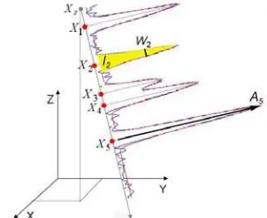
Let us assume that full waveform LIDAR data have been captured in a region of interest (ROI). A single waveform is decomposed by fitting a series of Gaussian pulses to the waveform which contains NR reflections (Figure 2).
Figure 2. 3D points and attributes derived from a waveform
The vector T ( , , , , )( 1,..., )
i x y z W Ii i i i i i NR
X is provided for each
reflection i with (xi,yi,zi) as the 3D coordinates of the
reflection. Additionally, the points Xi are given the width
2
i i
W σ and the intensity Ii 2 σi Ai of the return pulse
with σi as the standard deviation and Ai as the amplitude of the
reflection i (Reitberger et al., 2006; Jutzi and Stilla, 2005). Note that basically each reflection can be detected by the waveform decomposition. This is remarkable since some conventional LIDAR systems have a dead zone of about 3 m which makes these systems effectively blind after a reflection.
The sensor data are calibrated by referencing Wi and Ii to the
pulse width e
W and the intensity e
I of the emitted Gaussian pulse and correcting the intensity with respect to the run length
si of the laser beam and a nominal distance s0. Note that the correction assumes a targetsize larger or equal to the footprint (Wagner et al., 2006). The points from a waveform are subdivided into 4 point classes depending on the number of reflections within a waveform (Table 1).
Class Single First Middle Last
Table 1. Subdivision of points into classes in dependence on the number of reflections NRand the position i of the reflection in
the waveform
2.2 Singe tree detection
2.2.1 Watershed transformation
The first coarse detection of single trees is achieved from CHM by watershed transformation. The CHM is derived by subdividing the ROI into a grid having a cell spacing of cp and
NC cells. Within each grid cell, the highest 3D point is extracted
and adapted with respect to the ground level zgroundj , i.e. estimated from a given DTM by bilinear interpolation. In the next step, all the highest 3D points
)
width gw. For this purpose a method called ‘gridfit’ (D’Errico,
2006) is adopted which smoothens the surface by keeping the surface gradients as small as possible. The trade-off between interpolation and regularization is determined by the adjustable smoothing factor. Both steps are carried out simultaneously in a least squares adjustment. The result is a smoothed CHM having equally spaced cells. The watershed segments derived on this CHM act as candidate regions where single trees could be contained. The results can also be improved by an additional stem detection method to further detect small trees which are not represented by local maximums.
2.2.2 Normalized cuts segmentation
Within every watershed segments the new 3D segmentation technique using normalized cuts (Shi and Malik, 2000) is used to detect point clouds associated to single trees (Figure 3). This makes it possible to detect also smaller trees in th understory which cannot be indicated by local maxima in the CHM. This segmentation uses the positions (xi, yi, zi) of the laser reflections and optionally the pulse width Wi and the intensity Iiof the waveform decomposition. Additionally, stem positions or local maximums derived by the watershed segmentation of CHM can be used as prior knowledge. The normalized cut segmentation applied in the voxel structure of a (merged) watershed segment is based on a graph G. The two disjoint segments A and B of the graph are found by minimizing the cost function:
( , ) ( , ) ISPRS Annals of the Photogrammetry, Remote Sensing and Spatial Information Sciences, Volume I-7, 2012
the weights of all edges ending in the segment A. The weights
wij specify the similarity between the voxels and are a function of the LiDAR point distribution and features. A minimum solution for Eq.(3) is found by means of a corresponding generalized eigenvalue problem (Reitberger et al., 2009). It turned out that the spatial distribution of the LiDAR points mainly influences the weighting function. The features derived from the LiDAR points attributes from Wi and Ii only support in second instance the segmentation result. Note that the 3D segmentation approach is not dependent on full waveform LiDAR data. It can also successfully be applied to conventional LiDAR data just providing 3D point coordinates.
Figure 3. Single tree segmentation using normalized cut with the reference trees as black lines.
2.3 Feature extraction
Deriving significant features describing each tree individually is a key step in the classification of tree growing condition. The single tree detection provides for each segmented tree corresponding laser points. Crown points can be separated from possible existing stem reflections by finding the crown base height. All the laser hits above the crown base height form the crown points.
Based on our previous work (Reitberger et al., 2008), the six-group salient features Stree={Sg, SI, SW, Sn, Sf SC} of a tree can
be defined to reflect the tree geometric and physical properties. The features will be defined as follows, respectively, while the detailed definition of the first four features can be referred to the Reitberger et al. (2008):
S
S }, which describe the outer tree geometry. The
first feature 1
g
S comprises two curvature parameters of a parabolic surface fitted to the crown points. The second parameter 2
g
S records the mean distances of points in all equidistance height-layers to the tree stem position.
SI ={ 1
I
S , 2
I
S }, which describe the tree reflectional properties against laser beam, which benefits from intensity information provided by the waveform decomposition. The first feature 1
I
S
computes the mean values of laser points in each height layer. The second parameter 2
I
S is introduced as overall mean intensity value for the entire tree segment.
SW ={ c
mean
S }, which uses the pulse width information provides for each point from waveform decomposition. However, the definition of this feature is limited to the single und first pulses, which could lead to a distinct broadening effect of pulses. Sn ={ 1
n
S ,Sn2}, where
1
n
S is the average number of reflections between the first and last reflection in the waveform for laser shots with multiple reflections, 2
n
S is the proportion of the number of laser shots with single reflections to the number of laser shots with multiple reflections for the tree segment.
S
S }, which is designed to characterize the gap fraction of single trees. The gap fraction is usually not directly measurable from laser scanning, and therefore, is here approximated by two features. The first feature 1
f
S is derived as the ratio of below canopy echoes to the total number of echoes. The threshold for confining the canopy echoes is set to 1m above ground. The second feature 2
f
S is parameterized as an echo ratio defined as
2
f
S =(nfirst+ nintermediate)/( nlast+ nsingle) (4) where n is the respective number of echoes per tree segment plus below ground echoes. If no last and single echoes are found within a cell, the echo ratio is set to 1, indicating a dense vertical extension and low transparency of the tree object. SC ={ d
C
S ,SCV}, where d C
S is the maximal diameter of the tree crown, V
C
S is the volume of the tree crown derived based on 3D alpha shape. The tree crowns are extracted from single 3D tree segments.
2.4 Discrimination between dead and living trees
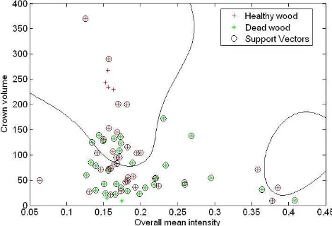
Tree growing conditions are distinguished between dead and living trees by a supervised classification using support vector machine (SVM) technique. SVM is utilized owing to its computational simplicity and superior accuracy. It is not constrained to prior assumptions on the distribution of input data and is, hence, well suited for complex feature space, e.g. nonlinear recognition problems. The SVM was originally designed for binary classification; therefore, in this study, the binary SVM is directly implemented for our task in a genuine way (dead and living trees) without handling the multiclass problem. Moreover, the RBF kernel is used here. In addition, the kernel based implementation of SVM needs to select multiple controlling parameters, including the kernel parameters, etc. In our case, these parameters were selected automatically based on the LOO (leave-one-out) algorithm (Chapelle et al., 2002). It is based on the idea that the expected generalization error is to be minimized where the optimization of the parameters is carried out by a gradient descent search over the parameter space. The most important parameters to try search are box constraint for soft margin and sigma value for RBF kernel. After obtaining a reasonable initial parameter, they can be refined to get better accuracy. An example of 2D feature map with SVM is depicted in Figure 4.
Figure 4. 2D feature space as an example to undergo SVM classification of discriminating between dead and living trees, the black lines indicate the SVM nonlinear decision boundaries ISPRS Annals of the Photogrammetry, Remote Sensing and Spatial Information Sciences, Volume I-7, 2012
3. EXPERIMENTS 3.1 Material
Experiments were conducted in the Bavarian Forest National Park which is located in south-eastern Germany along the border to the Czech Republic (49o 3’ 19” N, 13o 12’ 9” E). 2 sample plots with an area size between 1000 m2 and 3600 m2 were selected in the mixed mountain forests. The plots comprise forest in the regeneration phase, the late pole phase. The test sites have suffered from tree disease due to bark beetle attack. Reference data for all trees with diameter at breast height (DBH) larger than 7 cm have been collected in May 2006 and 2007 for 247 Norway spruces (Picea abies), 63 European beeches (Fagus sylvatica), 3 Sycamore maples (Acer pseudoplatanus) and 1 Tilia. Several tree parameters like the DBH, total tree height, stem position and tree species were measured and determined with the help of GPS, tacheometry and the ’Vertex’ III system. A DTM with a grid size of 1 m and an absolute accuracy of 25 cm was available.
Plot Size [ha]
Altitude
[m] Trees/ha
Deciduous [%]
Mortality [%]
21 0.2 860 500 66 20~30
59 0.1 810 2150 1 35~40
Table 2. Characteristics of sample plots
Full waveform data have been collected by Milan Flug GmbH with the Riegl LMS-Q560 scanner in May 2006 after snowmelt but prior to foliation and in May 2007 after foliation with an average point density of 25 points/m2(Table 3). The vertical sampling distance was 15 cm, the pulse width at half maximum reached 4 ns and the laser wavelength was 1550 nm. The flying altitude of 400 m resulted in a footprint size of 20 cm.
Time of flight May ‘2006 May ‘2007
Foliage Leaf-off Leaf-on
Scanner Riegl LMS-Q560 Riegl LMS-Q560
Pts/m2 25 25
AGL [m] 400 400
Footprint [cm] 20 20
Table 3. Configurations for two airborne LiDAR campaigns
3.2 Calibration
The calibration of the Riegl full waveform system was determined from special calibration flights performed over an airfield. Several tracks were flown at different flying heights (200 m and 400 m) along and across the airfield. The mean intensity Ii, corrected with respect to the emitted intensity Ie, and the mean run length si were calculated in four homogeneous areas (122 m2–133 m2) for each track.
Flight 2006 Flight 2007
Calibrated parameter k 1.902 1.736 Table 4 Estimation of calibration parameter k
According to Eq. (2), the best coefficient k was estimated from all possible observation equations
k k
i i j j
I s I s (5) which can be formulated for two tracks i and j flown at different heights. Table 4 shows the results obtained for the two flights of data sets.
3.3 Single tree detection
The procedures for 3D single tree detection were applied to the plots in a batch procedure without any manual interaction. Table 5 contains the percentage of detected trees for two plots. The trees are subdivided into 3 layers with respect to the mean height htop of the 100 highest trees per ha. The lower layer
contains all trees below 50 % of htop, the intermediate layer
refers to all trees between 50 % and 80 % of htop, and, finally,
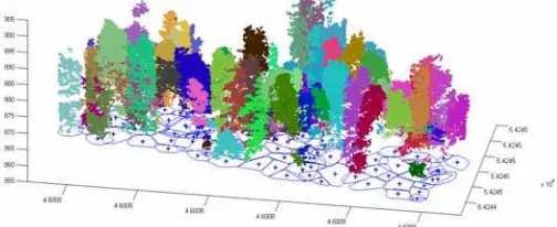
the upper layer contains the rest of the trees. Figure 5 shows a sample area containing several coniferous trees. The tree tops derived from the local maximums of the CHM correspond in some cases with the reference trees reasonably. The tree detection results were evaluated by comparison with reference data using two criterions: i). the distance of detected trees should be smaller than 60% of the mean tree spacing of the plot; ii) the height difference between detected and reference trees should be smaller than 15% of htop. If a reference tree is
assigned to more than one tree position, the tree position with the minimum distance to the reference is selected. Detected trees that are liked to one tree position are so-called “detected trees” and detected trees without any link to a tree position are treated as “false positives”.
Figure 5. Single tree detection of sample area with 3D segments, the outlines and positions of single trees are projected onto the x-y plane
Data
set Correctly detected trees per height layer [%] False
pos [%] lower intermediate upper total
2006 61 69 75 70 23
2007 59 70 73 67 25
Table 5. 3D Detection of single trees in the reference plots
The overall detection rate of up to 70 % can be achieved for our experiments, while up to a quarter of the detection corresponds to false alarm. It can be indicated that most of the trees are detected in the upper layer. In comparison, in the intermediate and lower layer the detection rate is relatively smaller. However, the innovative tree detection method based on 3D segmentation has fully exploited advantages of full waveform data to detect small trees. Most of dominate trees in the middle and lower layer have been detected, yielding much better results than previous studies, even better than ours presented in Reitberger et al. (2009). One of the important reasons is that we have a generous horizontal threshold for matching reference trees. The number of false detected trees indicates a moderate reliability. Additionally, if we compare data set I (leaf-off) to dataset II (leaf-on) it can be addressed that the foliage condition could affect the detection rate, but not significantly. As expected, the overall detection rate is worse by ca.3% in leaf-on situation, while the false positive has increased by 2%. It could be caused by the reason that dense tree crowns in leaf-on condition hinder the detection or dead woods have emerged in the meantime.
3.4 Classification of dead and living trees
A binary SVM classification is applied to correctly detected trees to distinguish between dead and living ones based on various features defined for single trees. A 5-fold cross validation is performed in order to fairly assess the results and minimize the impact of the selection of training data.
The numbers in the Table 6 refer to the classification results using various combinations of features. The results show that the classification works best with a combination of all features. It seems that there are no unique single features working best for both datasets. However, as unexpected, the features SI SW describing the physical reflection properties have constantly a less positive effect on both datasets, independent of the foliage conditions. Moreover, the features Snand Sf dedicated to the
penetration behavior of laser pulses influence the classification accuracy significantly in the leaf-on case (dataset II). Meanwhile, the features related to the outer geometry of crowns
g
S and Sc also perform better in the leaf-on case. Such facts
lead to the better overall accuracy in the leaf-on case than the leaf-off case. Finally, we combined all of the single features, which provided the lowest total classification error of 34% and 30% for the leaf-off/on cases, respectively. Tables 7 shows additionally the confusion matrices of the best classification results. A good overall accuracy of 73% is achieved for the leaf-on case, whereas only a moderate value can be obtained.
Feature Misclassification rate (%)
Leaf-off Leaf-on
g
S 42 35
I
S 45 47
W
S 45 45
n
S 50 41
f
S 40 41
SC 41 42
I W
S S 40 40
C g
S S 43 41
f
n
S S 47 37
2
g I W n f C
S S S S S S 34 30
Table 6 5-fold cross-validation results of SVM classification of dead and living trees using different combinations of tree segment features, the misclassification rate measures the proportion of misclassified observations of both classes.
Leaf-off Leaf-on
Living Dead Living Dead
Living 127 16 89 32
Dead 46 25 25 62
Overall accuracy 71% 73%
Kappa 0.27 0.45
Table 7 Confusion matrix of the best classification result for both datasets using 5-fold cross-validation
Furthermore, we show the distribution of the detected and reference living and dead trees for different DBHs in Figures 6 and 7. Note that the number of trees presented in these two
figures refers to the results of single tree detection rather than that of SVM classification. Therefore, only the capability of 3D tree segmentation with respect to dead woods detection is shown here.
Figure 6. Distribution histogram of detected and reference trees according to the DBH – leaf-off dataset
Figure 7. Distribution histogram of detected and reference trees according to the DBH – leaf-on dataset
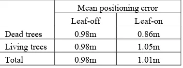
Mean positioning error
Leaf-off Leaf-on
Dead trees 0.98m 0.86m
Living trees 0.98m 1.05m
Total 0.98m 1.01m
Table 8. Accuracy of the tree position determination
Finally, Table 8 shows the absolute positional accuracy of the detected trees after classifying them into living and dead ones. Interestingly, the mean positioning error of dead trees in the leaf-on case gets better by 10 %, which corresponds to ca. 19 cm. In the leaf-off case, it seems to indicate no difference between dead and living trees. However, the overall accuracy of tree position determination is still better in the leaf-off condition.
4. DISCUSSION
Conceptually, the presented approach to detect dead wood from airborne LIDAR data of forest areas goes one step further than tree species classification. To the best of our knowledge, this paper presents the first complete scheme for detecting dead woods at single tree level using high density full waveform LiDAR data in forestry areas. In this study, based on the 3D single tree segments derived automatically in advance the classification of tree health states using waveform-laser measurements is performed. The 3D segmentation for single tree detection by normalized cuts could improve the detection rate in the lower forest layer by averagely 20% compared to 2D segmentation performed on the CHM. Moreover, the leaf-off case seems to be a more appropriate acquisition time for single ISPRS Annals of the Photogrammetry, Remote Sensing and Spatial Information Sciences, Volume I-7, 2012
tree detection in mixed mountain forests, since the segmentation of deciduous trees is more difficult due to considerable overlapping of adjacent trees.
When viewing at the results of the dead wood classification we obtained an overall accuracy up to 73% for both flight campaigns. The good results are provided mainly by waveform-specific features Sf describing the penetration ability of laser
pulses against tree crown in leaf-off and by Sgdescribing the
outer tree geometry in leaf-on case. In general, there is no unique feature which decisively contributes to the success of the classification of tree heath condition. The combined set of all features shows the best classification performance independent of the foliage condition. Furthermore, contrary to most of reported tree species classifications the leaf-on situation in our study is more favourable towards identifying dead trees from living ones than leaf-off case. It could be caused by different reasons. Firstly, under leaf-on condition the crown of deciduous trees exhibits a more abundant type, which leads to a stronger evidence for differing from coniferous dead trees making the distinction of tree types based on crown geometry and transmittance easier. Secondly, the leaf-on dataset used in this study was acquired one year later than the leaf-off data. Many dead trees have emerged within this time interval owing to the attack of bark beetle. This can also be retrieved from Figures 6 and 7, where reference dead trees have increased and reference living trees have decreased, especially for trees with small stem diameter. The analysis of the waveform data by Reitberger et al. (2008) shows that the intensity and pulse width indicate the best discrimination between the stem and crown points. Dead trees should have mainly consisted of laser reflections from the stem and branch, which contribute to a high mean intensity value. However, intensity related featuresSI,SW show unexpectedly only moderate results for detecting dead woods in both datasets. It could be due to the reason that the mixed mountain forest composed of different tree species could oversmooth such intensity difference between tree crown and stem. Additionally, tree crown points which actually belong to adjacent trees could weaken the feature functions, even leading to worse overall classification results. Such false points could happen to the tree segments owing to tolerant threshold for selecting correctly detected trees.
5. CONCLUSIONS
The study presents a scheme for discriminating dead standing trees from living ones in forest areas based on a 3D single tree detection method from full-waveform LiDAR data. The results attained in heterogeneous forest types in different foliage conditions show that the overall accuracy and position of single trees independent of heath state could be obtained in a promising way. Based on the combinational analysis of waveform-specific, transmittance and geometric features defined at single tree level a clear dependency of the intensity and the pulse width towards the discrimination of tree health has not been found as it was expected. In contrary, features related to outer geometry seem to more contribute to the success of the classification. Future research could be focussed on assessing the influence of tree species on the classification of dead and living trees, since the mean intensity for single points is clearly different for coniferous and deciduous tree stems according to our previous study. Furthermore, the intensity difference between stems of living and dead trees needs to be examined, whether proving direct clues to discriminating the tree heath conditions.
REFERENCES
Bater, C W., Coops, N C., Gergel, S E., LeMay, V., Collin, D., 2009, Estimation of standing dead tree class distributions in northwest coastal forests using lidar remote sensing. Canadian Journal of Forest Research, 39(6) 1080-1091.
Chapelle, O., Vapnik,V., Bousquet, O., and Mukhherjee, S., 2002, Choosing multiple parameters for support vector machine, Machine Learning, 46 (1-3), 131–159.
D’Errico, 2006 D’Errico, J., 2006, Surface fitting using gridfit. http://www.mathworks.com/matlabcentral/fileexchange(accessd on 10.01.2009)
Jutzi B., Stilla U. 2005. Waveform processing of laser pulses for reconstruction of surfaces in urban areas. In: Moeller M, Wentz E (eds) 3th International Symposium: Remote sensing and data fusion on urban areas, URBAN 2005. International Archives of Photogrammetry and Remote Sensing. Vol 36, Part 8 W27.
Kim, Y.,Yang, Z.,. Cohen, W. B., Pflugmacher, D., Lauver, C. L., Vankat, J. L., 2009, Distinguishing between live and dead standing tree biomass on the North Rim of Grand Canyon National Park, USA using small-footprint lidar data, Remote Sensing of Environment, 113(11), pp.2499-2510.
Korpela, I., Ørka, H.O., Maltamo, M., Tokola T., & Hyyppä J., (2010). Tree species classification using airborne LiDAR – effects of stand and tree parameters, downsizing of training set, intensity normalization, and sensor type. Silva Fennica, 44(2): 319–339.
Pasher, J., King, D J., 2009, Mapping dead wood distribution in a temperate hardwood forest using high resolution airborne imagery. Forest Ecology and Management, 258(7), pp.1536-1548.
Pyysalo, U., Hyyppä, H., 2002. Reconstructing Tree Crowns from Laser Scanner Data for Feature Extraction. In ISPRS Commission III, Symposium 2002 September 9 - 13, 2002, Graz, Austria, pages B-218 ff (4 pages).
Reitberger, J., Krzystek, P., Stilla, U., 2008 Analysis of full waveform LIDAR data for the classification of deciduous and coniferous trees. International Journal of Remote Sensing, 29(5): 1407-1431
Reitberger, J., Schnörr, Cl., Krzystek, P., Stilla, U., 2009. 3D segmentation of single trees exploiting full waveform LIDAR data, ISPRS Journal of Photogrammetry and Remote Sensing, 64(6), pp.561-574
Shi, J., & Malik, J., 2000, Normalized cuts and image segmentation. IEEE Transactions on Pattern Analysis and Machine Intelligence, 22, 888 – 905.
Solberg, S., Næsset, E., Hanssena, K H., Christiansena E., 2006, Mapping defoliation during a severe insect attack on Scots pine using airborne laser scanning. Remote Sensing of Environment, 102(3-4), pp. 364-376.
Solberg, S., Naesset, E., Bollandsas, O. M., 2006. Single Tree Segmentation Using Airborne Laser Scanner Data in a Structurally Heterogeneous Spruce Forest. Photogrammetric Engineering & Remote Sensing, Vol. 72, No. 12, December 2006, pp. 1369-1378.
Stilla, U., Yao, W., Jutzi, B., 2007, Detection of weak laser pulses by full waveform stacking. In: Stilla U, et al (eds) PIA07 Photogrammetric Image Analysis 2007. International Archives of Photogrammetry, Remote Sensing, and Spatial Information Sciences, Vol 36(3/W49A):25-30
Wagner, W., Ullrich, A., Ducic, V., Melzer, T. and Studnicka, N., 2006, Gaussian decomposition and calibration of a novel small-footprint full-waveform digitising airborne laser scanner. ISPRS Journal of Photogrammetry and Remote Sensing, 60, pp. 100-112.
Yao, W., Stilla, U., 2010, Mutual Enhancement of Weak Laser Pulses for Point Cloud Enrichment Based on Full-Waveform Analysis. IEEE Transactions on Geoscience and Remote Sensing, 48(9), pp.3571-3579. Yu, X., Hyyppa, J., Vastaranta, M., Holopainen, M., & Viitala, R., 2011, Predicting individual tree attributes from airborne laser point clouds based on the random forests technique. ISPRS Journal of Photogrammetry and Remote Sensing, 66(1), pp.28-37 ISPRS Annals of the Photogrammetry, Remote Sensing and Spatial Information Sciences, Volume I-7, 2012