Electronic Journal of Qualitative Theory of Differential Equations 2007, No.13, 1-14;http://www.math.u-szeged.hu/ejqtde/
Computation of radial solutions of semilinear
equations
Philip Korman
Department of Mathematical Sciences University of Cincinnati
Cincinnati Ohio 45221-0025
Abstract
We express radial solutions of semilinear elliptic equations on Rn
as convergent power series inr, and then use Pade approximants to compute both ground state solutions, and solutions to Dirichlet prob-lem. Using a similar approach we have discovered existence of singular solutions for a class of subcritical problems. We prove convergence of the power series by modifying the classical method of majorants.
Key words: Semilinear elliptic equations, Pade approximants, convergence of solutions.
AMS subject classification: 65L10, 35J60.
1
Introduction
exact computations, see e.g. O. Aberth [1]. In this work we develop series approximations of radial solutions of semilinear elliptic equations onRn.
There is a lot of interest in the radial solutions of semilinear problems of the type
∆u+f(u) = 0,
both on balls in Rn, and on the entire space. With r = |x|, and together
with initial conditions, the equation becomes
u′′+ n−1
r u′+f(u) = 0
(1.1)
u(0) =u0, u′(0) = 0,
and we wish to compute the solution as a power series inr, for any initial value of u0. We begin by showing that the power series solution contains
only even powers of r, i.e. u(r) = Σ∞
i=0air2i, with a0 = u0. We then
de-rive a recursive formula forai, which is easy to implement in Mathematica.
One can quickly compute a lot of terms of the series, giving highly accu-rate approximation for smallr, practically an exact solution. The problem is that the power series solution usually has a finite radius of convergence, which can be small (if f(u0) is large). We need another approximation of
solutions, which is defined for allr, and which agrees with the power series approximation for small r. A classical way of doing so is to use Pade ap-proximations. These are rational functions, whose power series expansion agrees, as far as possible, with that of the function being approximated, see e. g. G. A. Baker [2]. We found this approach to be remarkably successful, providing us with practically closed form solutions for both Dirichlet prob-lem, and ground state case. It is important for us that highly accurate Pade approximants are provided byMathematica, with just two easy commands.
majorization of solutions of (1.1) by solutions of certain first order equation.
Using a similar approach we have discovered existence of singular positive solution for the problem
u′′+n−1
r u
′+λu+up= 0, u′(0) = 0, u(1) = 0
not only in the supercritical range p > nn+2−2, which is well known (see F. Merle and L. A. Peletier [6]), but also for subcriticalp’s, satisfyingp >nn
−2,
which is rather surprising. We obtain the singular solution in the form
u(r) = r−2/(p−1)Σ∞
i=1air2i, and compute the unique λ = ¯λ at which this
solution occurs. Our computations indicate convergence of the above series for smallr >0, but we did not carry out the proof.
2
Series solution
Letu=u(r) be a radial solution of the initial value problem
u′′+ n−1
r u′+f(u) = 0
(2.1)
u(0) =u0, u′(0) = 0,
wheref(u)∈C∞[0,∞), andu
0 >0. It will be convienient for us to consider
solutions of (2.1) for both positive and negativer, even though one usually has r ≥ 0 for the polar coordinate r. We wish to compute the solution as a series nearr = 0, i.e. u(r) = Σ∞
i=0biri. The following lemma shows that
bi= 0 for all oddi.
Lemma 2.1 Any solution of the problem (2.1) is an even function.
Proof: Even though the initial value problem has a singularity atr = 0, it was shown in L. A. Peletier and J. Serrin [7] that it has the properties of regular initial value problems, in particular there is uniqueness of solutions to (2.1) for small|r|. We may also consider solutions of (2.1) in case r <0. Observe that the change of variables r → −r leaves (2.1) invariant. If solution was not even, we would have two different solutions of (2.1) for
r >0, contradicting the just mentioned uniqueness result. ♦
In view of the lemma, we may express the solution of (2.1) as u(r) = Σ∞
u(r) = Σki=0air2i, which we expect to provide us with a solution, up to the
terms of orderO(r2k+2). Write
(2.2) u(r) = ¯u(r) +akr2k,
where we regard ¯u(r) as already computed, and the question is how to get
ak. (We begin with ¯u(r) = u0.) If we plug our ansatz (2.2) into (2.1), we
and on the surface it may appear that we need to solve a nonlinear equation forak. It turns out that we can get an explicit formula forak. Express
Observe that when we repeatedly apply the L’Hˆopital’s rule, all terms in-volving ¯uwill vanish, and we have
lim
We arrive at an explicit formula for the coefficients:
(2.5) ak=−
i=1air2i. The repeated differentiations in (2.5) can be easily
performed using symbolic software likeMathematica. (Actually, Mathemat-ica is able to compute limr→0 f(¯u(r))+¯u
′′+n−1 r u¯′
r2k−2 too, in case u0 is rational,
presumably by using the above formula.)
Example We have solved the problem
u′′+3 ru
and obtained a series solution, corresponding to a known explicit ground-state solution u(r) = 8+8r2.
We got lucky in this example. After computing a series solution, we have identified the sum of the series, u(r) = 8+8r2. This function gives solution
of the problem for all r > 0, while the corresponding series has radius of convergence√8. In general, the sum of a series solution cannot be identified, and moreover the radius of convergence may be small (iff(u(0)) is large). The problem is that power series approximation has a limited range. We need another approximation of u(r) = 8+8r2, which is defined for all r. A
classical way is to use Pade approximations.
3
Pade approximations
ExampleWe have solved the problem
u′′+2 ru
′+u5= 0, u(0) = 1, u′(0) = 0.
It is connected to the previous example in the sense that they both give radial solutions of the critical PDE, with applications to geometry,
∆u+unn+2−2 = 0,
wherenis the dimension of the space. (We use series to solve serious PDE’s.) Similarly to the previous example, we wish to compute the ground-state solution. We computed a series solution, which begins with
(3.1) u(r) = 1−1 6r
2+ 1
24r
4
−4325 r6+ 35 10368r
8
−69127 r10+. . . .
It seems unlikely that one can identify the sum of this series through ele-mentary functions (even though there is a closed formula for this sum, which we mention below). After computing 55 terms of this series (powers of up tor110), we have used a built inMathematica command to approximate this polynomial of power 110 by its Pade approximation, centered atr= 0, and using polynomials of power 50 for both the numerator and denominator of Pade approximation. We called this rational approximation p(r). To see how well it approximates the solution, we plugged it into our equation, and considered the “defect”
q(r)≡p′′(r) +2 rp
20 30 40 50 60r 2·10-6
4·10-6 6·10-6 8·10-6 q
Figure 1: The defect of Pade approximation
10 20 30 40r
0.2 0.4 0.6 0.8 1 p
Figure 2: Pade approximation of the solution
The graph ofq(r) is given in Figure 1. One can see thatq(r) is small. It gets even smaller forr >60, and it is practically zero whenr∈(0,10). We see thatp(r) is an excellent approximation to the solution. The graph ofp(r)
is given in Figure 2. This problem has an exact solution, u(r) =
√
3
√
3 +r2.
We used it to confirm both the validity of the series (3.1), and the accuracy of the Pade approximants (this accuracy can be improved, increasing powers of both numerator and denominator, with the power of denominator chosen larger than numerator to allow decay to zero for larger).
RemarkThere is a closed form solution for the critical initial value problem
u′′+n−1
r u
′+unn+2−2 = 0, u(0) =α, u′(0) = 0.
It isu(r) =α
n(n−2)
n(n−2) +α4/(n−2)r2
n−22
, see e.g. [8] or [5]. Our previous
0.6 0.7 0.8 0.9 r 0.0001 0.0002 0.0003 0.0004 q
Figure 3: Defect of the approximation of the solution
The same approach works equally well for Dirichlet problems.
Example On a unit ball inR3 we consider a sub-critical problem
(3.2) ∆v+v4 = 0, for|x|<1, v = 0 when|x|= 1.
By the classical results of B. Gidas, W.-M. Ni and L. Nirenberg [4] the problem (3.2) has a unique positive solution, which is moreover radially symmetric, i.e. u = u(r), where r = |x|. It follows that (3.2) may be replaced by the ODE
(3.3) v′′+2 rv
′+v4= 0, v′(0) = 0, v(1) = 0.
We begin by solving the initial-value problem
u′′+2 ru
′+u4 = 0, u(0) = 1, u′(0) = 0.
Similarly to the previous example, we have computed 55 even terms of the power series approximation at r = 0, and then approximated this polyno-mial of power 110 by its Pade approximation, centered at r= 0, and using polynomials of power 50 for both the numerator and denominator of Pade approximation. We used this approximation of u(r) to find its first root
R≈14.9716. Then by standard scaling,v(r) =R2/3u(R r) gives an approx-imation to the solution of (3.3). To see how good is this approxapprox-imation, we again computed q(r) = v′′ +2
rv′+v4. In Figure 3 we give the graph
of q(r), which shows that the accuracy is high. (q(r) is even smaller when
r∈(0,0.6).) In Figure 4 we graph the approximation ofv(r).
4
Analyticity of solutions
conver-0.2 0.4 0.6 0.8 1 r 1
2 3 4 5 6 v
Figure 4: Solution of the Dirichlet problem (3.2)
gence (evaluatingak+1/ak for largek allows one to approximate the radius
of convergence). In this section we prove convergence of the series solution for the problem (2.1), with any realn≥1.
We begin by showing an alternative derivation for the coefficients of the series solution. We rewrite the equation (2.1) as
(4.1) ru′′+ (n−1)u′+rf(u) = 0, u(0) =u
0, u′(0) = 0.
Differentiating,
ru′′′+nu′′+f(u) +rf′(u)u′ = 0
Setting r = 0, we express u′′(0) = −1
nf(u0). Differentiating (4.1) three
times, we can express u′′′′(0), and in general, differentiating 2k−1 times,
we express
(4.2) (n+ 2k−2)u(2k)(0) =−(2k−1) d
2k−2
dr2k−2f(u(r))|r=0,
which means that the coefficients of the Maclauren series for u(r), a2k = u(2k)(0)
(2k)! , are the same as given by (2.5).
In the numerical examples above, solution was given by alternating power series. The following result describes a class of f(u), for which this is true. (We do not claim yet that the series is convergent.)
Theorem 4.1 Assume that fk(u) >0 for all k ≥0 and u > 0. Then the coefficients of the series solution are alternating.
Proof: Suffices to show that the series solution has positive coefficients inξ=−r2. Making this change of variables in (2.1), we have
(4.3) 4ξuξξ+ 2nuξ=f(u), u(0) =u0 >0, uξ(0) =
1
Differentiating the equation (4.3), and setting ξ = 0, the way we just did, we see that Ddξkku(0) > 0 for all k ≥ 1, and hence the Maclauren series for u(ξ) has all of its coefficients positive. ♦
We recall the classical notion of majorizing series. Let u(r) = Σ∞
k=0ukrk
Then it has a majorant of the form sCs −r.
Proof: Since the series Σ∞
k=0uksk converges, we can find a constant C,
so that |uk|sk ≤ C. This means that the series u(r) = Σ∞k=0ukrk has a
majorant Σ∞
k=0sCkrk= sCs−r. ♦ Theorem 4.2 Assume that f(u) is a real analytic function. Then the so-lution of the problem (2.1), with any real n≥1, is analytic, i.e. the series u(r) = Σ∞
k=0
u(2k)(0)
(2k)! r2k, where u(2k)(0) are computed using formula (4.2), converges for smallr.
(Observe that v(i)(0) >0 for all i≥ 1, as follows by the differentiating of (4.6), since the function sCs
−v has positive derivatives.) To calculateu (m)(0),
we differentiate (4.4) m−1 times and set ξ= 0, obtaining
(4m−4 + 2n)u(m)(0) = Σ∞ same type of a sum, involving v and its derivatives at r = 0. Using our inductive hypothesis and (4.5), we conclude the claim (4.7).
We claim that solution of (4.6) is in turn majorized by the solution of the first order problem
provided that we increaseC (if necessary, and the increase is made in both (4.8) and (4.9)) so that the value ofwξ(0) computed from (4.9),wξ(0) = 2Cn,
By the inductive hypothesis the right hand side here is greater than that in (4.8) (both involve only positive terms), and hencev(m)(0)≤w(m)(0) for all m≥1.
Finally, we explicitly integrate the equation (4.9), obtaining
w(ξ) =s−
r
s2− Cs n ξ,
which can be represented by a convergent power series for smallr (since the binomial series converges for smallr). ♦
5
Application to singular solutions
We consider positive solution of the Dirichlet problem on a unit ball inRn
(5.1) ∆u+λu+up= 0, for|x|<1, u= 0 on|x|= 1.
Here λ is a positive parameter, and p > 1. It is well known that when
p > nn+2−2, the critical exponent, there is a unique ¯λ at which a singular solution exists, see F. Merle and L. A. Peletier [6]. Moreover, the significance of the critical solution is by now well understood: the curve of positive solutions of (5.1) tends to infinity, asλ→λ¯, and it approaches the singular solution for r 6= 0. Using power series expansion, we show that there is a unique ¯λ at which a singular solution exists for p > nn−2, i.e. for some sub-critical equations too.
It is easy to see that a singular solution must blow up like r−p−21 near r= 0. We denote θ=−p−21, andA=−θ(n+θ−2). Observe thatA >0 if and only ifp > nn−2. We shall obtain a solution of (5.1) in the form
(5.2) u(r) =r−p−21v(r),
wherev(r)∈C2[0,1) satisfies
(5.3) v(0) =Ap−11.
We assume thatn≥3, andp > nn−2. In casep < n+4n we assume additionally that (this assumption is not needed ifp≥ n+4n )
(5.4) 2i(2i+n+ 2θ−2) + (p−1)A >0 for all integers i≥1.
Observe that (5.4) gives a finite set of conditions, since the conditionp > nn−2
implies that θ > −n+ 2, and then (5.4) holds if i > n−2
2 . If we assume a
stronger condition p ≥ n+4n (which is larger than n−2
2 for n ≥ 4), then θ >−n/2, and the condition (5.4) holds. Since n+4n < nn+2
−2, we see that the
condition (5.4) is satisfied for supercriticalp.
Radial solutions of (5.1) satisfy
(5.5) u′′+ n−1
r u
′+λu+up = 0, forr <1, u(1) = 0.
Using the ansatz (5.2) in (5.1), we see thatv(r) satisfies
(5.6) r2v′′+ (n−1 + 2θ)rv′+
θ(n+θ−2) +λr2
We are looking for a solution of (5.6) satisfying
(5.7) v′(0) =v(1) = 0.
We now scaleλout of (5.6), by letting r= √1
λξ. Then v(ξ) satisfies
(5.8) ξ2v′′+ (n−1 + 2θ)ξv′+
−A+ξ2
v+vp = 0,
and d v
d ξ(0) = 0. Setting here ξ= 0, we see that v(0) satisfies the condition
(5.3). Hence this condition is necessary for existence of singular solution. We shall produce a power series solution of (5.8).
The equation (5.8) can be considered for ξ <0 too. Since this equation is invariant under the transformation ξ → −ξ, it follows that any classical solution is an even function, and so its power series expansion contains only even powers. We then look for solution of (5.8) in the form
(5.9) v(ξ) = Σ∞
i=0aiξ2i.
Plugging into (5.8), we have
(5.10) a0+ Σ∞i=1ciξ2i+ a0+ Σ∞i=1aiξ2i
p
= 0,
where
(5.11) ci = [2i(2i+n+ 2θ−2)−A]ai+ai−1.
The constant terms in (5.10) will vanish if we choosea0 =A 1
p−1. We show
that setting the power ofξ2i to zero produces a linear equation fora
i of the
form
(5.12) [2i(2i+n+ 2θ−2) + (p−1)A]ai+g(a0, a1, . . . , ai−1) = 0,
whereg is some function of previously computed coefficients. (Actual com-putations are easy to program, using Mathematica.) Indeed, denoting t = Σ∞
i=1aiξ2i, we rewrite the last term in (5.10) as
a0+ Σ∞i=1aiξ2i
p
=ap0Σ∞
j=0
p j
tj aj0 .
The term ξ2i with a coefficient involving a
i occurs when j= 1 in this sum,
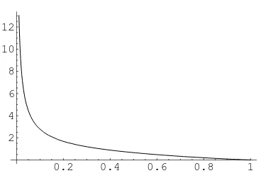
0.2 0.4 0.6 0.8 1 2
4 6 8 10 12
Figure 5: Singular solution of the problem (5.13)
Assume we could prove convergence of the series (5.9). (Our computa-tions strongly suggest convergence.) This would give us solution for small
ξ. Standard existence result gives us solution for all ξ. It is easy to see thatv(ξ) will eventually vanish. (v′′(0) = 2a
1 <0, sov(ξ) is decreasing for
small ξ. By maximum principle solution cannot turn around, and hence it tends to zero. Thenvp term is negligible, andv(ξ) can be expressed through Bessel functions.) Let γ denote the first root of v(ξ). Then ¯λ = γ2, and
u(r) =rθv(γr) is the singular solution of (5.8) atλ= ¯λ.
Example If n = 3, then nn+2−2 = 5 and n−n2 = 3, n+4n = 7/3. We took a subcriticalp= 4, and found that the singular solution of
(5.13) u′′+n−1
r u
′+λu+u4 = 0, forr <1, u(1) = 0
occurs at ¯λ≃5.26295. Here are the first few terms of the singular solution
u(r)≃r−2/3(0.60571−0.79695r2+ 0.18236r4+ 0.02615r6 −0.02201r8
+0.00471r10+ 0.00054r12).
Its graph is shown in Figure 5. When we plugged this solution into (5.13) at
λ= ¯λ, we obtained the left hand side practically zero for allr∈(0,1). If the reader wishes to compute this solution using a standard ODE solver, he can start with u(1) = 0, u′(1)≃ −0.836857, and solve the equation (5.5) (with λ= 5.26295) for decreasingr over (0,1). (Or one can start withu(−1) = 0,
u′(−1) ≃ 0.836857, and solve the equation (5.5) forward for −1 < r < 0,
sinceu(r) is an even function.)
References
[1] O. Aberth, Precise numerical methods using C++. With 1 CD-ROM (Windows 95). Academic Press, Inc., San Diego, CA, 1998.
[2] G. A. Baker, Jr. and P. Graves-Morris, Pad´e Approximants. Second edition. Encyclopedia of Mathematics and its Applications, 59. Cam-bridge University Press, CamCam-bridge, 1996.
[3] C. Budd and J. Norbury, Semilinear elliptic equations and supercritical growth, J. Differential Equations 68no. 2, 169-197 (1987).
[4] B. Gidas, W.-M. Ni and L. Nirenberg, Symmetry and related properties via the maximum principle,Commun. Math. Phys.68, 209-243 (1979).
[5] I. Flores, A resonance phenomenon for ground states of an elliptic equa-tion of Emden-Fowler type, J. Differential Equations 198 no. 1, 1-15 (2004).
[6] F. Merle and L. A. Peletier, Positive solutions of elliptic equations in-volving supercritical growth, Proc. Roy. Soc. Edinburgh Sect. A 118, no. 1-2, 49-62 (1991).
[7] L. A. Peletier and J. Serrin, Uniqueness of positive solutions of semi-linear equations in Rn, Arch. Rational Mech. Anal. 81, no. 2, 181-197
(1983).
[8] X. Wang, On the Cauchy problem for reaction-diffusion equations,
Trans. Amer. Math. Soc. 337, no. 2, 549-590 (1993).
[9] P. Zhao, and C. Zhong, Positive solutions of elliptic equations involving both supercritical and sublinear growth, Houston J. Math. 28 no. 3, 649-663 (2002).