FEATURE DESCRIPTOR BY CONVOLUTION AND POOLING AUTOENCODERS
L. Chen, F. Rottensteiner, C. Heipke
Institute of Photogrammetry and GeoInformation, Leibniz Universität Hannover, Germany - (chen, rottensteiner, heipke)@ipi.uni-hannover.de
Commission III, WG III/1
KEY WORDS: Image Matching, Representation Learning, Autoencoder, Pooling, Learning Descriptor, Descriptor Evaluation
ABSTRACT:
In this paper we present several descriptors for feature-based matching based on autoencoders, and we evaluate the performance of these descriptors. In a training phase, we learn autoencoders from image patches extracted in local windows surrounding key points determined by the Difference of Gaussian extractor. In the matching phase, we construct key point descriptors based on the learned autoencoders, and we use these descriptors as the basis for local keypoint descriptor matching. Three types of descriptors based on autoencoders are presented. To evaluate the performance of these descriptors, recall and 1-precision curves are generated for different kinds of transformations, e.g. zoom and rotation, viewpoint change, using a standard benchmark data set. We compare the performance of these descriptors with the one achieved for SIFT. Early results presented in this paper show that, whereas SIFT in general performs better than the new descriptors, the descriptors based on autoencoders show some potential for feature based matching.
1. INTRODUCTION
Feature based image matching aims at finding homologous feature points from two or more images which correspond to the same object point. Key point detection, description and matching among descriptors form the feature based local image matching framework, e.g. (Lowe, 2004). The performance of local image matching is determined to a large degree by an appropriate selection of a descriptor. For each key point to be matched, such a descriptor has to be extracted from the image patches surrounding the key-point, and these descriptors can be seen as features providing a higher-level representation of the key point. In this context, hand-crafted features such as SIFT (Lowe, 2004) and SURF (Bay et al., 2008) have been shown to be very successful in image matching. However, the manual feature design process, also referred to as feature engineering, is labor intensive and thorny. In order to make an algorithm less dependent on feature engineering, it would be desirable to learn features automatically. As a by-product, one can hope that based on automatically learned features, novel applications can be constructed faster (Bengio, 2013).
Bengio et al. (2013) claim that artificial intelligence must understand the world as it is captured by the sensor. They argue that this can only be achieved if one can learn to identify and disentangle the underlying explanatory factors hidden in the observed low-level sensor data. To learn features automatically from low-level sensory data rather than designing features manually can be seen as an attempt to capture the explanatory factors directly from the data. Recent progress in feature learning (Farabet et al., 2013) has shown that the application of automatically learned features can lead to comparable or even better results than using classical manually designed features in image classification.
Feature-based image matching also relies on an appropriate selection of features (descriptors) rather heavily, whilst only a quite limited number of studies about feature learning has been conducted in this community. In our previous work (Chen et al., 2014), we learned a descriptor as well as the corresponding
matching function based on Haar features and Adaboost classification, relying on labeled (matched or unmatched) image patch pairs. This work was based on supervised learning. In order to be able to learn descriptors without having to provide manually annotated training data, in this paper we use unsupervised learning algorithms, in particular autoencoders for that purpose. Thus, we will for the first time apply this framework, originally designed for image encoding and classification tasks, to the problem of feature based matching. We will introduce three ways in which this can be achieved. The focus of this paper is on the comparison of the new methods with each other, but also with the classical hand-crafted descriptor provided by SIFT, in order to show the potential, but also the limitations of such an approach.
2. RELATED WORK
Classical hand-crafted descriptors, e.g. SIFT (Lowe, 2004) and SURF (Bay et al., 2008), aggregate local features in a window surrounding a key-point. An extension of SIFT is given by PCA-SIFT (Ke and Sukthankar, 2004), which introduces dimension reduction of SIFT by analyzing the principal components of SIFT descriptors over a large number of SIFT descriptors which are extracted from real images. Other hand-crafted feature descriptors all inherit the spirit of aggregating local feature response but vary the shape of pooling from grid (SIFT) to log-polar regions (Mikolajczyk and Cordelia, 2005) or concentric circles (Tola et al., 2010).
Building a descriptor can be seen as a combination of the following building blocks (Brown et al., 2011): 1) Gaussian smoothing; 2) non-linear transformation; 3) spatial pooling or embedding; 4) normalization. If we take corresponding image patch pairs from different images as positive matching samples, image matching can be dealt with as a two-class classification problem. For the input training patch pairs, the similarity measure based on every dimension of the descriptor is built. Fed with training data, the transformation, pooling or embedding The International Archives of the Photogrammetry, Remote Sensing and Spatial Information Sciences, Volume XL-3/W2, 2015
that gets minimum loss can be found to build a new descriptor (Brown et al., 2011).
Early descriptor learning work aimed at learning discriminative feature embedding or finding discriminative projections, while still using classic descriptors like SIFT as input (Strecha et al., 2012). More recent work deals with pooling shape optimization and optimal weighting simultaneously. In (Brown et al., 2011), a complete descriptor learning framework was presented. The authors test different combinations of transformations, spatial pooling, embedding and post normalization, with the objective function of maximizing the area under the ROC curve, to find a final optimized descriptor. The learned best parametric descriptor corresponds to steerable filters with DAISY-like Gaussian summation regions. A further extension of this work is convex optimization introduced in (Simonyan et al., 2012) to tackle the difficult optimization problem in (Brown et al., 2011).
Since descriptor is naturally a kind of representation for the raw input data, it holds an innate link to representation learning, where researchers try to teach an algorithm how to extract useful representations of the raw input data for applications such as image classification (Farabet et al., 2013). The unsupervised learning method we use in this paper, autoencoders (Hinton and Zemel, 1994), tries to find interesting structures in the raw input data by minimizing a reconstruction error of the input data. To the best of our knowledge, current work on descriptor learning concentrates on supervised learning side, while there is a lack of work on using unsupervised determine a feature descriptor. Each image patch is normalized to zero-mean and unit-variance in advance, which can reduce the effect of radiometric distortions.
3.1 Basic Structure
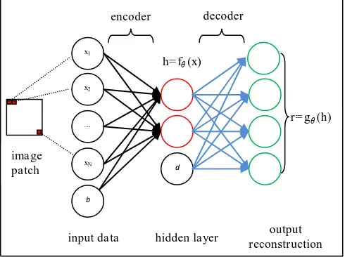
An autoencoder is a specific form of a neural network (NN). Generally, a neural network contains one input layer, optionally one or more hidden layers, and one output layer. Each layer is composed of several units. For example, the NN shown in Figure 1 consists of one input layer, one hidden layer and one output layer. The number of units in the input layer depends on the input data and the number of units of the output layer equals to the number of target variables, e.g., the number of categories in image classification.
In a NN, connections can be added between units of the same layer or between units of different layers. The most commonly used structure only connects the units in one layer with units in its neighboring layer. Except for units of the input layer, each unit will compute the weighted sum of all its inputs coming from units of the previous layer, where the weights are learned parameters. After adding a bias value to the weighted sum, a non-linear activation function is applied to generate the output of the unit, which, in turn, can be the input to a unit of the next layer. This non-linear activation function improves the modeling ability of neural networks. Otherwise, the combination of multiple layers would just be equivalent to using
a one-layer linear mapping. The different layers of the network apply a series of linear and non-linear transformations to the input data. These transformations gradually transform the input data to the higher level output representation in a nested functional form.
The feature extraction function fθin an autoencoder, also called
encoder, is defined explicitly in a specific parameterized closed form. A feature vector can be computed as h= fθ(x) from an input x with a form fθ(x)=(b+ Wex), where is the logistic sigmoid function, serving as the activation function (Ng, 2011):
1 vector h corresponds to the output of the hidden units in the NN and x corresponds to input units as shown in Figure 1. Note here the input x corresponds to a square image patch of size K x K, whose grey values are arranged in a column vector as shown in Figure 1. Every pixel in image patch corresponds to one element in the vector x. The matrix We corresponds to the weights of the connections corresponding to the black arrows in Figure 1 connecting the input and the hidden layers. Thus, a linear mapping via the encoder weight matrix We and bias b is first computed, then the non-linear sigmoid function is applied to this mapping. The feature vector h is the result of the autoencoder that will be used to define a descriptor that should be a high-level representation of the image patch. Each line j in the weight matrix We contains the weights for all the inputs of the corresponding element hj in the feature vector. As the input units correspond to a quadratic image patch, each line j of the weight matrix can be interpreted as containing the coefficients of a convolution filter applied to that image patch, and the output of that filter is the feature hj. The fact that the weights We are learned from the data means that in fact the convolution filter that forms the basis of feature extraction is learned. This is also true for the bias values that form the second input for the non-linear transformation via the sigmoid function.
Figure 1. The Autoencoder's architecture. Input, hidden and output units are indicated by black, red and green
circles, respectively.
blue arrows in Figure 1, are the decoder weight matrix and bias, respectively. The autoencoder tries to approximate the input x with the reconstructed signal r. Here r corresponds to the output units, as shown in Figure 1. The training data consist of image patches of size K x K in image patches surrounding key points determined using some key-point extractor; details of training data generation is described in section 6. Here we suppose the number of training examples (image patches) is m. By subtracting the reconstruction r from the input x and applying the Euclidean norm to this difference over all training samples we can get the reconstruction error L(x, r). In order to learn the parameters of the autoencoder, i.e., the weight matrices and biases of both the encoder and the decoder, this error function has to be minimized. To prevent overfitting, a regularization term is also added to the Euclidean norm of the difference. The overall cost function is (Ng, 2011):
2 m = number of training samples
N = K x K = number of units of the input layer x H = dimensionality of h
λ = weight parameter
The weight parameterλcontrols the relative importance of the regularization term compared to the reconstruction error term. One can learn the parametersθ= {We, b, Wd, d} of the encoder and the decoder simultaneously by minimizing the cost function J(). Obviously, if the encoded feature h has the same dimensionality as the input data x, the encoder will be the identity function. In this case, it will be meaningless. To get interesting structure inside the input data x, the structure of the auto-encoder system should be constrained. The first constraint normally used, as indicated in Figure 1, is that the dimensionality of the encoded feature h should be low. If there are structures in x, some of these structures will be discovered by such a model (Ng, 2011).
Another constraint is the sparsity constraint. Sparsity means that most of the hidden units (learned feature vector components) stay "inactive", i.e., give an output close to 0 when presented with an input x. In particular, for a specific hidden unit j, we first denote its average (over the training data) activation (Ng, 2011) as:
= average activation of the hidden unit j j = index of hidden unit
= activation function of the hidden unit j
The enforced sparsity constraint (Ng, 2011) is:
j
(4) Here ρ is a constant, typically a small value, e.g. 0.05. This implies that we would like the average activation of the hidden neurons to be close to . To satisfy this constraint, the hidden units’ activations must mostly be near 0 (Ng, 2011).
An extra penalty term considering the sparsity constraint is added to the const function in Equation 2 (Ng, 2011):
(KL) divergence. Minimizing the KL-divergence will cause
j autoencoder by minimizing the cost function J’(θ) in Equation 6. For that purpose we use gradient descent based on the limited-memory Broyden–Fletcher–Goldfarb–Shanno method (Møller, 1993; Ng, 2011), which requires the partial derivatives of the
2. Compute the errors of each unit in the output layer. 3. Back-propagate the errors to each hidden unit 4. At each unit, use the corresponding activation extraction; for that purpose, we use the Difference of Gaussian (DoG) detector, which is scale-invariant (Lowe, 2004). For each detected feature point, we extract an image patch centered at
that point and aligned with the feature point’s main direction,
which is determined in the way described in (Lowe, 2004). The size of the image patch is selected to be four times the extracted
point’s scale. This image patch is resampled to a square of P x P pixels, where P is a parameter selected by the user. The second parameter is the size of the image patch that defines the number of input units for the autoencoder. This input is based on a patch of K x K pixels. The variants of the descriptor differ in the relation between P and K:
1) K < P: In this case, the K x K support region for the autoencoder can be shifted within the P x P image patch. In The International Archives of the Photogrammetry, Remote Sensing and Spatial Information Sciences, Volume XL-3/W2, 2015
this case, the autoencoder is applied to several K x K sub-windows in the larger image patch, and the descriptor is derived from all autoencoder outputs; there are two versions of the descriptor that are based on different strategies for selecting sub-windows and for generating the actual descriptor
2) K = P: in this case one can directly use the autoencoder output as the descriptor for the interest point.
To train the autoencoder, the DoG interest point detectors is applied to training images, the P x P support regions are extracted as described above, and each potential K x K sub-window is extracted. All of these sub-sub-windows are collected as the final training patches.
4.1 Descriptor DESC-1: K < P, no pooling
In this situation, the image patches extracted near a feature point are larger than the area for applying autoencoder, so that the autoencoder is applied to four sub-windows of the P x P image patch. The arrangement of these sub-windows is indicated by squares of different colour in Figure 2. Please note that the four sub-windows will overlap. We concatenate the hidden outputs of the learned autoencoder in these four sub-windows from left to right, top to bottom, to get a descriptor, whose dimension will be 4 x H, where H is the dimension of the feature vector h of the autoencoder. This descriptor will be referred to as DESC-1 in our experiments.
Figure 2. The arrangement and size (in pixel) of DESC-1. The learned autoencoder is applied to each of the 4 coloured regions, and the resulting feature vectors are concatenated to form the final key point descriptor.
4.2 Descriptor DESC-2: K < P, pooling is applied
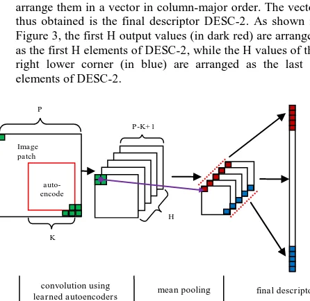
Alternatively, the autoencoder can be applied to each potential K x K sub-window of the P x P pixels. If we just concatenate the hidden output of these units as in DESC-1, we will get descriptor of a much higher dimension. To make things worse, many components of such a descriptor will be redundant and thus might hurt the discriminative power of the descriptor. To avoid this redundancy, we introduce a feature pooling strategy (Brown et al., 2011). Specifically, to produce DESC-2 the following steps are carried out (cf. Figure 3):
1) We apply the autoencoder to each possible sub-window inside the image patch. The size of the autoencoder window and the image patch is K× K and P× P pixels, respectively.
Using the short-hand D = P-K+ 1, there are D x D such windows. For each such window we determine H features. Consequently, we obtain H maps of D x D pixels each.
2) We apply mean pooling to the resultant maps: Each map is split into non-overlapping sub-windows of C × C pixels,
and the average value of each map is computed for each of these sub-windows. This results in H. output maps of size (D/C) x (D/C). This step is illustrated by the purple arrow in Figure 3 for one of the sub-windows of size C x C.
3) We take the values at each location in these maps and arrange them in a vector in column-major order. The vector thus obtained is the final descriptor DESC-2. As shown in Figure 3, the first H output values (in dark red) are arranged as the first H elements of DESC-2, while the H values of the right lower corner (in blue) are arranged as the last H elements of DESC-2.
Figure 3. The procedure of building DESC-2.
The dimensionality of DESC-2 is (D/C)×(D/C)×H.
4.3 Descriptor DESC-3: K = P
In this situation, the autoencoder is directly trained based on the resampled P×P patches. The H hidden values of the learned
encoder is directly arranged as a vector to give the final descriptor DESC_3. Consequently, the descriptor will have H dimensions.
5. DESCRIPTOR EVALUATION FRAMEWORK
To evaluate the performance of our descriptors, we rely on the descriptor evaluation framework in (Mikolajczyk and Schmid, 2005). We use their online affine datasets1. As the images in the datasets are taken either from planar scenes or from the same sensor positions just using rotated cameras, image pairs are always related by a homography. Every sub-dataset contains six images transformed to different degrees, and the homography between the first image and the remaining five images in each sub-dataset is provided with the dataset. The datasets include six types of transformations, namely rotation, zoom + rotation, viewpoints changes, image blur, JPEG compression, and light change. One test image pair for 'viewpoint change' is shown in Figure 4.
5.1 Data generation
After applying the DoG detector to the test images, we extract image patches surrounding feature points in the way described in Section 4. After that, our descriptors are extracted from these
1
http://www.robots.ox.ac.uk/~vgg/research/affine/ (accessed 10 February 2015)
Image patch
convolution using
learned autoencoders mean pooling final descriptor P
P-K+ 1
H
K auto-encode
r
K
K K
P
patches, and the nearest neighbor matching strategy is used to get correspondence between patches from different images. We use the nearest neighbor distance ratio to eliminate unreliable matches, i.e. matches for which the ratio between the distances of the two nearest neighbors in descriptor space is smaller than a threshold (Lowe, 2004; Mikolajczyk and Schmid, 2005).
Figure 4. One test image pair from "graf" datasets.
The ground truth correspondences are produced according to the ratio of intersection and union of the regions surrounding a key point (Mikolajczyk and Schmid, 2005). In short, if two detector regions share enough overlap after projecting into one image using the homography, these two key points are judged to be a correspondence. Just as (Mikolajczyk and Schmid, 2005), we also set the minimum overlap ratio required for a point pair to be considered to be a correct match to 0.5.
5.2 Evaluation criteria
Following the work in (Mikolajczyk and Schmid, 2005), we use recall and 1-precision as evaluation criteria. The recall is defined as follows:
#
. #
correct matches recall
correspondences
(7)
where #correspondences is the number of ground truth correspondences that is generated according to procedures described in 5.1, whereas #correct matches is the number of correct matches from the matching result based on the descriptor to be evaluated. This criterion gives the proportion of all potential matches that are detected based on the descriptor. A perfect result would give a recall equal to 1, which means the tested descriptor can find all potential matches between the two tested images.
The second criterion is 1-precision, which is defined as the number of false matches divided by the total number of matches.
#
1 .
# #
false matches precision
correct matches false matches
(8)
For the interpretation of the figures and possible curve shapes please refer to (Mikolajczyk and Schmid, 2005). By varying the nearest neighbor distance ratio, one can get different recall and 1-precision values that are used to generate performance curve.
6. EXPERIMENTS
In this section, we first present our trained autoencoders for different values of K. By observing the training result we can see how the basic components of image patch (or sub-patch) changes with K. This part is covered in section 6.1. Afterwards, we present the performance evaluation of DESC-1, DESC-2 and
DESC-3 using different parameters over K, C and H in section 6.2. The comparison to SIFT is also presented in this section.
6.1 Trainging of Autoencoders
The training of the autoencoders is based on images from the Urban and Natural Scene Categories2 of the LabelMe dataset. The training data are generated as described in section 4.We randomly select 50 and 100 images from this dataset for the training of 1) and 2), respectively. After processing as described in section 4, the number of training patch is 78400 and 133164 for 1) and 2), respectively. For 3) and 4), we randomly select 400 images and obtain 178677 training patches. Our implementation is based on the Vlfeat library (Vedaldi and Fulkerson, 2010).
In all experiments, we use patches of 16 x 16 pixels for extracting the descriptors, thus P = 16. The parameters of the cost function minimized in the training procedure are set to
ρ=0.05, λ=0.0001. These values were found empirically. As far as the other parameters of the descriptors (K, H) are concerned, we use four different settings:
1) K = 9, H= 9; 2) K = 11, H= 12; 3) K = 16, H= 64; 4) K = 16, H= 128.
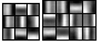
Obviously, variants 1) and 2) correspond to for DESC-1 and DESC-2, while 3) and 4) are relevant to define DESC-3. The autoencoder learning is implemented based on the exercise code from the Unsupervised Feature Learning and Deep Learning (UFLDL) online tutorial3. The trained auto-encoders for variants 1) and 2) are shown in Figure 5.
Figure. 5 Learned encoders of autoencoders. Left: setting 1); Right: setting 2)
In the left part of Figure 5, there are 9 K x K blocks for variant 1). Each of these blocks indicates the encoding weight between the K x K inputs and one of the hidden units. Consequently, each block shows one row of the weight matrix We of the autoencoder, which can be interpreted as a convolution filter of size K x K used to obtain one of the features of h. The interpretation of the weights for variant 2) on the right hand side of Figure 5 follows similar lines, the difference being that here we have H = 12 such convolution filters of size 11 x 11. The learned weights of the autoencoders are similar to convolution filters for detecting edges in images. However, using larger values of K and H, some of the learned convolution filters correspond to blob features, as shown in Figure 6. The results for variant 4) shows similar but more abundant relevant structures.
2
http://cvcl.mit.edu/database.htm (accessed 10 February 2015) 3
http://ufldl.stanford.edu/tutorial/unsupervised/Autoencoders/ (accessed 10 February 2015)
6.2 Performance Evaluation
Table 1 shows the image pairs used for performance evaluation in this paper. We select the first three images in every dataset as test images, and image matching are conducted between the first and the second (also third) image. By varying the nearest neighbor distance ratio from 1.2 to 3.2 we obtain the recall and 1-precision curve. The dominator on the label of vertical axis is the number of correspondences which are generated according to section 5.1.
Transformations Dataset Index of image pairs zoom + rotation "bark" 1-2, 1-3 viewpoint change "graf" 1-2, 1-3 image blur "trees" 1-2, 1-3 light change "leuven" 1-2, 1-3 JPEG compression "ubc" 1-2, 1-3
Table 1. Image pairs for performance evaluation.
Figure. 6 Learned encoders of autoencoders for setting 3)P = 16, K = 16, H= 64.
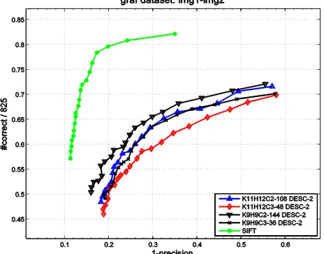
6.2.1 Different pooling size for DESC-2: We start with the evaluation of DESC-2, where we can use different sizes for pooling (described by the parameter C; cf. Section 4.2). With different pooling sizes, the dimensionality of DESC-2 will be different. We tested 4 different variants of DESC-2 as shown in Table 2.
Name K H C Dimensionality of descriptor
K11H12C2-108 DESC-2 11 12 2 108
K11H12C3-48 DESC-2 11 12 3 48
K9H9C2-144 DESC-2 9 9 2 144
K9H9C3-36 DESC-2 9 9 3 36
Table 2. Different pooling configurations of DESC-2.
The performance evaluation on the "graf" dataset of these descriptors from different configuration is given in Figure 7. Performance curves in other datasets all show a similar trend, they are not included here for lack of space. The performance of SIFT is also presented. The descriptor K9H9C2-144 DESC-2 performs best among those four configurations, but all learned descriptors perform worse than SIFT. One possible
interpretation of this could be that K9H9C2-144 DESC-2 has the highest dimensionality of the descriptor among the four descriptors.
Figure 7. Descriptor performance curves for different pooling configurations of DESC-2
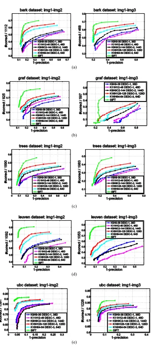
6.2.2 Comparison of DESC-1, DESC-2 and DESC-3: In this section we tested different variants of DESC-1, DESC-2 and DESC-3 as indicated in Table 3. For the descriptor type DESC-2, we only use the best one from section 6.2.1, K9H9C2-144 DESC-2.
Name K H C Dimensionality of descriptor
K9H9-36 DESC-1 9 9 ~ 36
K11H12-48 DESC-1 11 12 ~ 48
K9H9C2-144 DESC-2 9 9 2 144
K16H64-64 DESC-3 16 64 ~ 64
K16H64-128 DESC-3 9 128 ~ 128
Table 3. Different configurations for DESC-1, DESC-2 and DESC-3.
Figure 8 shows the performance evaluation result for of the different configurations for all types of transformation listed in Table 1.
From the performance curves shown in Figure 8 one can infer that all variants of DESC-1, DESC-2 and DESC-3 are currently inferior to SIFT in terms of recall and 1-precision.
6.3 Discussion
In all tested transformations, the DESC-3 descriptor performs better than DESC-1 and DESC-2. This superiority is much more distinctive in (a) zoom + rotation, (d) light change and (e) JPEG compression. Between the two DESC-3 descriptors, K16H64-128 DESC-3 is better than K16H64-64 DESC-3 almost in all cases. In the cases of (a) zoom + rotation, (b) viewpoint change and (c) image blur, DESC-2 performs much better than DESC-1. A potential explanation of this fact could be that the convolution (densely extracted redundant features) and pooling find more discriminative components in the whole patch since they try every potential sub-window while DESC-1 only uses four fixed sub-windows.
(a)
(b)
(c)
(d)
(e)
Figure 8. Performance curves of different descriptors under different types of transformations. (a) zoom + rotation. (b) viewpoint change. (c) image blur. (d) light change. (e) JPEG compression
Although our current result shows that DESC-3 is inferior to SIFT, from the comparison we can still have several interesting comments:
1) It is possible to improve the performance of the DESC-3 by increasing H. Currently, the maximum value for H used in our experiments is 128. Whether or not this can be improved further by increasing the dimensionality of the descriptor still needs to be studied.
2) The performance of all kinds of descriptors might be further improved by tuning the parameters both in autoencoder (N, H,λ, ρ) and the descriptor construction (K, H, C).
3) Adding a supervised framework which integrates descriptor learning and learning of the matching score function as it was carried out in our previous work (Chen et al., 2014) seems to be a natural extension of this work. In this context, the features to be learnt could be based on DESC-3. Another very important notable point of our work is that it the shift between the training data and performance evaluation data, that is to say, we train our descriptor on another data set than the test set. This is due to the fact that the performance evaluation data is a really small size dataset which cannot support a reasonable training of our encoder. Even though descriptors do not perform as well as SIFT, in particular DESC-3 seems to have the potential to achieve a performance good enough to be used for matching. This shows that unsupervised learning of descriptors for image matching based on autoencoders is feasible, though further research will have to show whether these preliminary results can be improved.
7. CONCLUSION
In this paper we have presented several types of descriptors based on learned autoencoders, which is an unsupervised learning algorithm. We evaluate the performance of these descriptors using the recall and 1-precision (Mikolajczyk and Schmid, 2005) curves. Evaluation results show that the present descriptor DESC-3 is the most promising one, and it may be possible to improve it both by tuning corresponding parameters and concatenating a supervised learning framework.
The future work will include more investigations into tuning the parameters of DESC-3. Furthermore, we will try to use more representative training data. Finally, we would like to integrate the unsupervised descriptor training with a supervised learning framework for additionally learning the matching score function.
ACKNOWLEDGEMENTS
The author Lin Chen would like to thank the China Scholarship Council (CSC) for supporting his PhD study in Leibniz Universität Hannover, Germany.
REFERENCES
Bay, H., Ess, A., Tuytelaars, T., et al., 2008. Speeded-up robust features (SURF). Computer Vision and Image Understanding, 110(3), pp. 346-359.
Bengio, Y. Courville, A. Vincent, P., 2013. Representation learning: A review and new perspectives. Pattern Analysis and Machine Intelligence, IEEE Transactions on, 35(8), pp. 1798-1828.
Bishop, C. M., 2006. Pattern recognition and machine learning. springer, New York, pp. 241-245.
Brown, M., Hua, G., Winder, S., 2011. Discriminative learning of local image descriptors. IEEE Trans Pattern Anal Mach Intell, 33(1), pp. 43-57.
Chen, L., Rottensteiner, F., & Heipke, C., 2014. Learning image descriptors for matching based on Haar features. ISPRS-International Archives of the Photogrammetry, Remote Sensing and Spatial Information Sciences, 1, pp. 61-66.
Farabet, C., Couprie, C., Najman, L., & LeCun, Y., 2013. Learning hierarchical features for scene labeling. Pattern Analysis and Machine Intelligence, IEEE Transactions on, 35(8), pp. 1915-1929.
Hinton, G. E. Zemel, R. S., 1994. Autoencoders, minimum description length, and Helmholtz free energy. Advances in neural information processing systems, pp. 3-3.
Ke, Y., Sukthankar, R., 2004. PCA-SIFT: A more distinctive representation for local image descriptors. Proceeding IEEE Conf. Computer Vision and Pattern Recognition, (2), pp. II-506-II-513
Mikolajczyk, K., Schmid, C., 2005. A performance evaluation of local descriptors. Pattern Analysis and Machine Intelligence, IEEE Transactions on, 27(10), pp. 1615-1630.
Møller, M. F., 1993. A scaled conjugate gradient algorithm for fast supervised learning. Neural networks, 6(4), pp. 525-533. LeCun, Y. Bottou, L. Bengio, Y. et al., 1998. Gradient-based learning applied to document recognition. Proceedings of the IEEE, 86(11), pp. 2278-2324.
LeCun, Y., Ranzato, M.A., 2013. Deep Learning Tutorial. International Conference on Machine Learning.
Lowe, D. G., 2004. Distinctive image features from scale-invariant keypoints. International Journal of Computer Vision, 60(2), pp. 91-110.
Ng, A., 2011. Sparse autoencoder. CS294A Lecture notes, 72. Rumelhart, D. E., Hinton, G. E., & Williams, R. J., 1988. Learning representations by back-propagating errors. Cognitive modeling, 5.
Simonyan, K., Vedaldi, A., Zisserman, A., 2012. Descriptor learning using convex optimisation. European Conference on Computer Vision (ECCV) 2012. Springer Berlin Heidelberg, pp. 243-256.
Strecha, C., Bronstein, A. M., Bronstein, M. M., Fua, P., 2012. LDAHash: Improved matching with smaller descriptors. IEEE Trans Pattern Anal Mach Intell, 34(1), pp. 66-78.
Tola, E., Vincent, L., Fua, P., 2010. Daisy: An efficient dense descriptor applied to wide-baseline stereo. IEEE Trans Pattern Anal Mach Intell, 32(5), pp. 815-830.
Vedaldi, A., Fulkerson, B., 2010. VLFeat: An open and portable library of computer vision algorithms. In Proceedings of the international conference on Multimedia ACM. pp. 1469-1472. The International Archives of the Photogrammetry, Remote Sensing and Spatial Information Sciences, Volume XL-3/W2, 2015