AIRBORNE LIDAR: A FULLY-AUTOMATED SELF-CALIBRATION PROCEDURE
S. M. Lindenthal a, b,*, V. R. Ussyshkin a,*, J.G. Wang b, M. Pokorny a
a Optech Incorporated, 300 Interchange Way, Vaughan, ON L4K 5Z8, Canada - (steffenl, valerieu, martinp)@optech.ca b Dept. of Earth and Space Science Engineering, York University, 4700 Keele Street, Toronto, ON M3J 1P3, Canada - (steffen,
jgwang)@yorku.ca
Commission VI, WG VI/4
KEY WORDS: LIDAR, Calibration, Laser Scanning, Classification, Point Cloud, Quality, Accuracy
ABSTRACT:
Automated calibration of LIDAR systems has been an active field of research and development over the last years. Traditional calibration approaches rely on manual extraction of geometric features in the laser data and require time-intensive input of a trained operator. Recently, new methodologies evolved using automatic extraction of linear features and planar information to minimize systematic errors in LIDAR strips. This paper presents a new methodology of LIDAR calibration using automatically reconstructed planar features. The calibration approach presented herein integrates the physical sensor model and raw laser measurements and allows for refined calibration of internal system parameters. The new methodology is tested and compared with a traditional approach based on manual boresighting using a typical survey mission. Optech’s software suite LMS, which is the first commercial implementation of this functionality, was used to process the data and to derive means of quality assessment. Different methods of reconstructing automatically extracted geometric features are presented and discussed in the context of their contribution to the calibration process. The final results are compared numerically and through graphic quality check.
* Corresponding author
1. INTRODUCTION
Applications in the fields of surveying, mapping, and GIS vary in regards to the level of precision and accuracy that is required. For planimetric maps at scales of 1/1000 and larger, high vertical accuracy of digital elevation datasets is necessary. In such survey applications, the requirements for LIDAR measurement accuracy are often a few centimetres to provide expected quality of LIDAR-derived end products. In order to meet stringent accuracy requirements and minimize systematic errors, it is essential to ensure proper calibration of the LIDAR sensor.
LIDAR systems are calibrated at the manufacturer site in lab and in-situ to minimize systematic errors. However, for a number of reasons (Schenk, 2001; Ussyshkin, and Boba, 2008; Habib, and Van Rens, 2008; Toth, and Shan, 2009; Vosselman, and Mass, 2010), sensor calibration provided by the manufacturer is not always stable enough to provide the required data accuracy. Some systems hold calibration better than others but it seems the calibration needs to be checked continuously. As a result, it is a common practice for LIDAR service providers to perform additional calibration procedures on a period basis. In large scale mapping applications with stringent accuracy requirements, additional system calibration is often required for every data collection mission.
Traditionally, service providers derive refined calibration parameters in an iterative procedure with manual adjustment of calibration parameters. It helps to minimize systematic errors and improve final data accuracy. However, it is a very time-consuming process requiring an experienced and skilful operator. Moreover, since LIDAR calibration is a complex multi-parametric task, manual approaches may not result in
proper system calibration. In addition, the lack of knowledge of system internal characteristics, which may affect system calibration, may lead to misinterpretation of the origin of systematic errors by system user. It may result in additional calibration errors rather than refined data and improved accuracy.
This paper presents a new, fully-automated, rigorous self-calibration technique that allows deriving a set of multi-parametric corrections with minimal input from the operator. It relies on automated rectification of sensor calibration parameters rather than manipulation of misaligned datasets. It will be shown that standard flight patterns and a few overlapping strips are sufficient for retrieving good calibration results, which make it suitable even for corridor surveys with no parallel or cross strips.
2. BACKGROUND: LIDAR CALIBRATION 2.1 System-based versus Data based Calibration
Over the last few years, various approaches of LIDAR self-calibration have been presented (Kager, 2004; Filin, and Vosselman, 2004; Friess, 2006; Skaloud, and Lichti, 2006; Habib et al., 2008; Rentsch, and Krzystek, 2009; Habib et al., 2010b). They differ with respect to how the observations are modelled, what parameters are being estimated, degree of automation and commercialization, required types of point classification. Some of the approaches seem to be more rigorous and robust than others. A detailed comparison of several new techniques, especially in regards to the parameters being estimated, is given in (Habib, and Van Rens, 2008).
The existing approaches can be classified into system driven and data driven methods (Habib et al., 2010a). Relying solely on the processed LIDAR point cloud, data-driven methods refine the xyz values without modifying sensor calibration parameters. Contrary, system-driven approaches relate sensor calibration parameters (which may or may not include internal sensor characteristics), directly to the measured coordinates of the laser points. Thus, xyz values are refined through improved sensor and installation parameter, which makes the calibration procedure more robust. some approaches create conjugate point correspondence indirectly either via generating TIN patches from the point cloud and establishing point-to-patch relations (Schenk et al., 2000; Habib et al., 2006; Pothou et al., 2007), or via organizing the data in raster structures and interpolating in both patches (Kraus et al., 2006). There is however the risk that TIN patches don’t represent the actual surface on the ground properly, which can cause the interpolated point coordinates to be biased and can transfer into degraded calibration results (Habib et al., 2010b).
Another popular strategy to deal with missing conjugate point redundancy is to extract planar segments or other geometric primitives from overlapping strips (Friess, 2006; Skaloud, and Lichti, 2006; Habib et al., 2008; Rentsch, and Krzystek, 2009). This approach has the advantage that raw observations can be used, however requires classification of laser points and use of additional parameters to model the geometric features. As long as the laser point cloud is biased by errors, neither tie points nor point-derived primitives coincide. Thus, refined calibration parameters are derived by minimizing the discrepancy between correspond-ding tie features in all categories of LIDAR calibration.
3. METHODOLOGY 3.1 Sensor-based Approach
The calibration methodology presented herein is based on automated rectification of sensor calibration parameters through extraction of planar segments from point cloud and using them as tie features. This methodology was introduced by Peter Friess (Friess, 2006) who further developed it into a fully-automated software tool. Recently it has become commercially available as Lidar Mapping Suite, LMS, in 2010. The crucial feature of LMS is a complete sensor mathematical model, which includes internal hardware characteristics affecting sensor calibration parameters. The discrepancies between tie features are minimized in a fully automated procedure of refining sensor calibration parameters. As a result, systematic errors are minimized and the data accuracy improved.
3.2 Extracting Tie Features
In traditional aerial triangulation, the first step is to lay out the imagery and orient the photos relative to each other. Corresponding points are utilized to tie the images together in a least squares adjustment that estimates corrections for the
orientation parameters of each image. Similar to the relative orientation in photogrammetry, the block geometry of the LIDAR survey is manifested in the dimensional arrangement of the laser swaths. To re-establish the geometry and topology of the point cloud, the laser points are organized in a cellular grid covering the whole survey area. To determine overlap, attributes are assigned in case that laser points from neighbouring strips fall within the same cell. In analogy to aerial triangulation, tie feature matching is the next steps to derive LIDAR calibration values.
3.3 Arranging Laser Points
Due to the irregular nature of LIDAR data, tie point matching in overlapping scan zones is not possible without interpolation. To solve for this, redundancy is generated indirectly and flight lines are searched for features that fulfil plane equations. If a plane is covered by more than one flight line, it can be used as tie feature. Each plane is characterized by a set of attributes: location of its centre point, slope, orientation and the fitting error (the fitting error describes the vertical distance to the adjusted plane of all laser points defining the plane). Based on these attributes, planes located within overlapping zones are tested for correspondence so to establish the link between identical planes.
Only a sub-set of planes is selected for the calibration process. Criteria are smoothness and low curvature, i.e. small point-to-plane distance, and variation in slope and orientation so to achieve increased de-correlation of system and plane parameters. Furthermore, sloped planes with small curvature are classified as roof planes. Roof peak lines are derived by intersecting adjacent roof planes with opposite orientation. A planar intersection is always feasible (Rentsch, and Krzystek, 2009) whereas spatial intersection is only possible if three or more neighbouring roof planes comrade. Practically, this means that often only horizontal intersection between estimated roof planes in overlapping strips are available for visual analysis. The computed roof peak lines serve as additional means to check the validity of the adjustment results.
3.4 Estimation of Plane and Calibration Parameters In aerial photogrammetry, the navigation solution and control and tie point measurements are integrated in a combined block adjustment to refine the position and orientation of the imagery. Camera calibration parameters and boresight angles between camera and IMU are usually estimated simultaneously. As in aerial triangulation, optimizing tie patches and system parameters is accomplished in a block adjustment that estimates corrections to reference plane parameters and relevant sensor and installation parameters simultaneously. However, there is a problem that many calibration parameters are highly correlated (ex: lever arm components between LIDAR and IMU, scan scale factor, and misalignment angles between LIDAR and IMU, drift parameters to compensate for drifts of the IMU gyros). Thus it is not recommended to estimate all parameters at the same time. To achieve good parameter de-correlation, it is further recommended to include a cross strip in the flight planning.
Algorithms correcting for the dimensional biases evolved more than a decade ago and are available nowadays in robust, commercial implementations. Procedures for estimating the angular misalignment of camera and IMU have been introduced over the last years (Cramer, 2001) and commercial solutions are well established (Kruck, 2006), too. Methods correcting for the
orientation biases between LIDAR and IMU however are still new (Skaloud, and Schaer, 2007; Ponthou et al., 2007). Similar to these methods, LMS also provides boresighting functionality based on the algorithms correcting dimensional biases.
In the course of this study it was established that grouping parameters and estimating one group of parameters at a time yields best results. For example, the parameter refinement process can be run twice so that each time some of the parameters to be optimized are kept fixed while others are adjusted. Table 1 gives an example of a typical combination for a single runs of parameter adjustment.
Sensor Boresighting mode
Production mode Scan angle offset Keep fixed Keep fixed Scan angle scale Free unknown Free unknown Scan angle lag Free unknown Free unknown Installation
Boresight angle Ex Free unknown Keep fixed Boresight angle Ey Free unknown Keep fixed Boresight angle Ez Free unknown Free unknown Position
Shift in X-coordinate Keep fixed Keep fixed Shift in Y-coordinate Keep fixed Keep fixed Shift in Z-coordinate Free unknown Free unknown Orientation
Roll correction Keep fixed Free unknown Pitch correction Keep fixed Free unknown Heading correction Keep fixed Keep fixed
Table 1. Typical settings for sensor and installation parameters adjustment entire mission. Roll, pitch and Z corrections are performed for each flight line. If no values from the prior mission are known, a first run with the “boresight” setup can be used to derive the start values for a refined production mode. The sensor and installation parameters can be estimated per instrument, per line, for the entire mission or a user defined area
3.5 Refined Point Cloud Computation
Based on the refined sensor, installation and plane parameters, the laser point cloud is re-computed. The planar surface and roof line estimates are updated and the finally derived parameters together with statistics and plots for quality assessment are generated. Several techniques established to judge the accuracy of the sensor calibration.
3.6 Accuracy Analysis
In aerial triangulation the internal accuracy, also referred to as relative accuracy or precision, is derived from the a posteriori variance factor and the variance-covariance matrix of the bundle block adjustment (Habib, and Van Rens, 2008). The external accuracy, also referred to as absolute accuracy, is obtained from check point analysis, where object points are re-calculated and
compared to their pre-surveyed reference coordinates (Cramer, 2001).
As raw LIDAR data however does not provide redundant (point) observations, a priori and a posteriori variance factor are identical. Quality measures need to be adapted as only the variance-covariance matrix is left as relative indicator of accuracy. Check planes can be utilized to assure that the estimated calibration parameters provide optimal internal accuracy, while tie planes cannot be used as check planes (Skaloud, and Lichti, 2006). The point-to-plane distance of all planar patches before and after adjustment can be used for quality check. Some specific features, like the offset of roof tops are used to characterize the mismatch between planes. Similarly, graphical display of roof ridge line pairs or complete roof profiles reveal spatial discrepancies and can be used to further analyze the relative accuracy of the data.
For absolute quality assessment the use of check points allows for absolute horizontal and vertical quality check. In case of LIDAR, special targets need to be deployed in the field though (Habib, and Van Rens, 2008). Alternatively, if prior knowledge of the survey area is available, pre-surveyed control patches can be utilized to verify the absolute accuracy of the estimated hardware parameters.
3.7 Iterative Process Flow
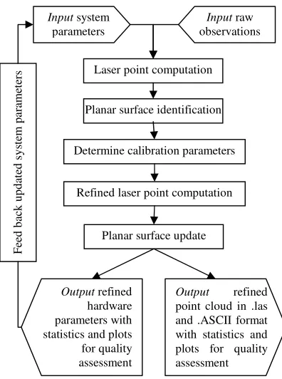
Figure 1 illustrates the overall process flow. Since the presented methodology relies on sequential refinement of selected sets of parameters, an iterative approach is essential to be implemented in the process flow.
Figure 1. Iterative refinement of parameters Laser point computation
4. FIELD TEST
The presented methodology was applied to a dataset collected by an ALTM-Orion system over downtown Toronto. An area extending approximately 5x3km with nine adjacent strips and one cross strip in the centre were selected for calibration (Figure 2). The data was collected at a height of 625m above ground with an average point density of 3 per square meter.
Figure 2. Flight lines displayed by GIS viewer
To extract planes within the selected block of data, the minimum number of points defining a plane was set to 12 and the maximum allowable point to plane distance was set to 25cm. The criteria for tie plane selection were a minimum of 20 points per tie plane, and a maximum fitting error of 15cm. Only plane pairs varying less than 20% in their number of points were included for deriving calibration parameters. The maximum separation between roof lines was set to 1 meter and the maximum azimuth difference between roof lines was limited to 1degree.
As this was the first time this system was flown on a survey, no flight-derived calibration values from prior surveys were available. In a standard calibration procedure, first-iteration set of calibration parameters is usually based on lab measurements, and the refined values would be derived after first calibration flight. In this case no lab-derived values were used for the first-iteration set of parameters and each one of the parameters was set to its default setting determined by the software. Table 2 shows some of the default settings used as initial system and installation parameters as the first-iteration set (“First Case”).
First case Second case Sensor corrections
Scan angle offset [deg] 0.0000 0.0000 Scan angle scale [-] 1.0000 1.1225 Boresight
Angle correction dEx [deg] 0.0000 0.0073 Angle correction dEy [deg] 0.0000 -0.0226 Angle correction dEz [deg] 0.0000 0.1300
Table 2. Initial system and installation parameter values
As the initial parameter values were expected to be far off from their final numbers, the focus of the “First Case” calibration was to retrieve a set of improved start values and to see how close these values would be to final calibration values. The parameter
estimates of the first calibration were then used as start values for a second calibration run ("Second Case") in order to test this procedure under usual conditions where previous calibration values would be on hand. The focus of the “Second Case” run was to test the robustness of this methodology and to see if the calibration results would converge towards similar end values.
Both cases were processed first in “boresight” mode to fix the angular misalignment between LIDAR and IMU and then in “production” mode to further refine the calibration parameter values. Particularly, it was expected that some of the boresight parameters might need rectification due to IMU drifts and other factors. Shift and drift parameters were determined individually for each line whereas corrections for angular mounting parameters were performed for the entire survey block.
5. RESULTS AND DISCUSSION
Within the calibration area, LMS identified about 2,500,000 tie planes and approximately 500,000 were selected for further processing. In Figure 3, extracted planes are depicted in light blue and planes selected for parameter estimation are depicted in dark blue. No planes could be located in the most southern lidar strip as this flight line covers the shore area of Lake Ontario.
Figure 3. Display of tie planes. Roof tops within the encircled area were used for further analysis
Figure 4 depicts the distance of LIDAR points to the estimated planes before and after rectification in the “First Case”. The distorted shape shown in Figure 4 (a) clearly indicates residual systematic errors, which is associated with poorly calibrated scale.
a
b
Figure 4. Point-to-plane distance before (a) and after (b) “First Case” rectification
Figure 4 (b) shows the same computation output after calibration parameter rectification. Based on the comparison between “First” and “Second” case start parameters (Table 2) one can conclude that the scanner scale value and a slight change in roll was indeed the main root cause of the systematic error evident in Figure 4(a). The graphical display of the point-to-plane distance after calibration turned out to be practically identical in both calibration runs. This is a good indication that the calibration parameters converged to correct final values despite the start scale value being far off.
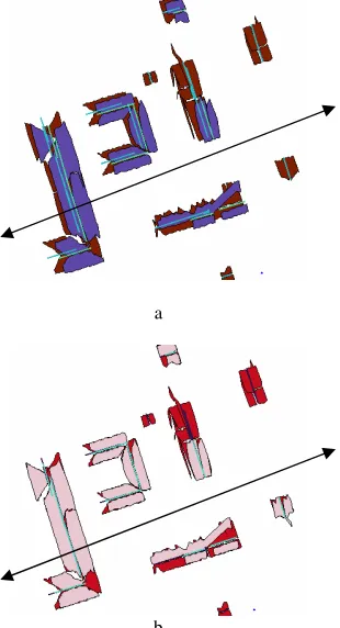
Figure 5 illustrates the quality check based on comparison of mismatches of roof lines in xy-plane.
a
b
Figure 5. Roof separation before (a) and after (b) “First Case” rectification. The double arrow indicates that the area was
scanned twice in opposite directions. Figure 4a (b) corresponds to Figure 5a (b)
Before calibration (Figure 5a), the roof ridge line separation was 1.5 m across flight-direction and 2 m in flight direction. As can be seen in Figure 5, the horizontal shift between the two scans can be related mostly to scale and pitch, as pitch causes separation in flight direction while a scale error results in discrepancy perpendicular to the flight direction. After successful refinement of installation parameters, the planimetric separation can be expected to be close to the tolerance level of the laser points on the ground. The remaining horizontal and vertical shifts are result in less than one decimetre difference on the ground. This however indicates that there are still some systematic errors remaining and that the initial calibration parameters were too far away to converge fully to its rectified final values.
To further refine the final calibration values gained from the first calibration run, the calibration cycle was repeated (“Second Case”). As mentioned previously, the point-to-plane distance graph (Figure 4b) turned out to look practically identical. The roofline separation however reduced further to only 2-3cm on the ground, which is near noise level of the laser measurements and confirms that the calibration values reached their final estimates. At this level of accuracy, using the roof plots for further visual analysis requires zoom and analyzing tolerance estimates and the magnitude of shift and drift parameters is a more efficient means of quality check. Considering the dynamics of the flight pattern and the GPS/IMU characteristics, the estimates of shift and drift parameters for each line are another means to judge the success of the calibration. Table 3 shows very small standard deviation values for roll and pitch for the final run, which indicates successful calibration. Moreover, standard deviations of elevation shifts (not shown in Table 3) were found to be smaller than 1cm in all cases.
Flight line
Roll deg
σ roll
deg
Pitch deg
σ pitch
deg
Z cor m
1 0.052739 0.001700 -0.01305 0.002025 -0.130
2 0.002401 0.000203 -0.01272 0.000903 0.069
3 0.003826 0.000197 -0.00095 0.000417 -0.003
4 0.005309 0.000146 -0.00038 0.000381 0.063
5 0.004776 0.000185 0.000249 0.000808 -0.028
6 0.000308 0.000172 0.009770 0.001132 0.003
7 0.005860 0.000212 -0.00541 0.000763 0.007
8 -0.00246 0.000169 0.005875 0.000584 -0.019
9 -0.00257 0.000265 -0.00362 0.000559 0.027
cross -0.00115 0.000106 0.001290 0.000251 0.012
Table 3. Roll, pitch and vertical shift estimates per flight line.
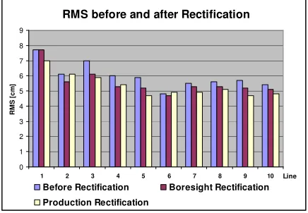
The final accuracy of the rectified laser point cloud was characterized by RMS values of the point-to-plain distance calculated by LMS for original and rectified datasets (Figure 6). Extensive testing and validation against control features has shown that the calculated RMS values (together with the a posteriori variance factor) are a true indicator of the absolute accuracy of the rectified laser point clouds. Based on the results presented in Figure 6, it was found that the elevation RMS improved by 6% during the “Second Case” calibration and had approached the typical limit determined by the random noise level. This is a clear indication that most systematic errors have been removed or significantly reduced during calibration process and the end parameter values represent true system calibration parameters. It is also important to note that both calibration runs, “First Case” and “Second Case” with poor and
refined start parameter values converged iteratively towards the same final values. It clearly indicates the robustness of the presented methodology and its applicability to various real-life scenarios.
RMS before and after Rectification
0 1 2 3 4 5 6 7 8 9
1 2 3 4 5 6 7 8 9 10 Line
R
M
S
[
c
m
]
Before Rectification Boresight Rectification
Production Rectification
Figure 6. RMS values before and after rectification
6. CONCLUSION
A new fully-automated LIDAR calibration methodology has been presented. It is based on iterative rectification of system-related calibration parameters minimizing discrepancies between planar tire features. As the result, systematic errors are reduced or eliminated. Control plane information can be integrated for absolute accuracy verification. It was shown that the new calibration methodology minimizes manual work and requires no special features to be designed to derive refine parameters and generate rectified data. The demonstrated results indicated robustness of the presented methodology and consistent improvement of final data accuracy.
7. REFERENCES
Cramer, M., 2001. Performance of GPS/Inertial Solutions in Photogrammetry, Photogrammetric Week, 2001, Stuttgart, Germany.
Filin S., and Vosselman, G., 2004. Adjustment of Airborne Laser Altimetry Strips. The International Archives of the Photogrammetry, Remote Sensing and Spatial Information Sciences, 35 (B3): pp. 285-289.
Friess, P., 2006. Towards a Rigorous Methodology for Airborne Laser Mapping, Proceedings of the International Calibration and Validation Workshop EURO COW, Castelldefels, Spain. Published as CD-ROM.
Habib, A.; Cheng, R.; Kim, E.; Frayne, M.; Ronsky, J. 2006. Automatic surface matching for the registration of LiDAR data and MR imagery. ETRIJournal, Vol. 28, No. 2. pp. 162-174.
Habib, A., Kersting, A. P., Ruifang, K., Al-Durgham, M., Kim, C., and Lee, D. C., 2008a. LiDAR strip adjustment using conjugate linear features in overlapping strips. Int. Arch. Photogramm. Remote Sens. Spat. Inf. Sci., 37 (part B1), pp. 385-390.
Habib, A., and Van Rens, J., 2008. Quality Assurance and Quality Control of LiDAR Systems and Derived Data, ASPRS 2008 Annual Conference, Portland, Oregon, April 28 – May 2, 2008.
Habib, A., Bang, K. I., and Kersting, A. P., 2010a. Lidar System Calibration: Impact on Plane Segmentation and photogrammetric Data Registration, ASPRS 2010 Annual Conference, San Diego, California, April 26 – May 30, 2010.
Habib, A., Bang, K. I., Kersting, A. P., and Chow, J., 2010b. Alternative Methodologies for LIDAR System Calibration,
Remote Sensing, ISSN 2072-4292, pp. 874-907.
Kager, H., 2004. Discrepancies between Overlapping Laser Scanning Strips- Simultaneous Fitting of Aerial Laser Scanner Strips. In: The International Archives of the Photogrammetry, Remote Sensing and Spatial Information Science, Istanbul, Turkey, Vol. XXXV, Part B/1, pp. 555 - 560.
Kraus, K., Ressl, C., and Roncat, A., 2006. Least Squares Matching for Airborne Laser Scanner Data, in: "Fifth International Symposium Turkish-German Joint Geodetic Days "Geodesy and Geoinformation in the Service of our Daily Life"", L. Gründig, O. Altan (ed.).
Kruck, E., 2006. Combined IMU Sensor Calibration and Bundle Adjustment with BINGO-F, OEEPE Official Publi-cation No. 43, “Integrated Sensor Orientation, Test Report and Workshop Proceedings”.
Ponthou, A., Toth C., Karamitsos S., and Georgopoulosv, A., 2007. On using QA/QC techniques for LiDAR/IMU boresight misalignment. MMT’07, “The 5th International Symposium on Mobile Mapping Technology”, Padova, Italy.
Rentsch, M. and Krzystek, P. (2009): Automatic Reconstructed Roof Shapes For LIDAR Strip Adjustment and Quality Control,
ISPRS Journal of Photogrammetry & Remote Sensing 61, 2009
Schenk, T., Krupnik, A., and Postolov Y., 2000. Registration of airborne laser data to surfaces generated by photogrammetric means. ISPRS, 32(3/W14), pp. 95-99.
Schenk, T., 2001. Modelling and Analyzing Systematic Errors in Airborne Laser Scanners. Technical Notes in Photogra-mmetry, The Ohio State University, Vol. 19, Columbus, USA.
Skaloud, J., and Lichti, D., 2006. Rigorous approach to bore-sight self-calibration in airborne laser scanning. ISPRS Journal of Photogrammetry & Remote Sensing, Vol. 61, pp. 47-59.
Skaloud, J., and Schaer, P., 2007. Towards Automated LIDAR Boresight Self-Calibration. MMT’07, “The 5th International Symposium on Mobile Mapping Technology”, Padova, Italy.
Toth, C. K., and Shan, J. 2009: Topographic Laser Ranging and Scanning, CRC Press, Chapter 4. LiDAR Systems and Calibration.
Ussyshkin, R.V., and Boba, M., 2008. Performance charac-terization of a mobile lidar system: Expected and unexpected variables, ASPRS 2008 Annual Conference, Portland, Oregon, April 28 – May 2, 2008.
Vosselman, G., and Maas, H.-G. 2010. Airborne and Terrestrial Laser Scanning, CRC Press, Whittles Publishing.