MINING CO-LOCATION PATTERNS FROM SPATIAL DATA
C. Zhoua,∗, W. D. Xiaoa,b, D. Q. Tanga,b
aScience and Technology on Information Systems Engineering Laboratory, National University of Defense Technology,
410073 Changsha, China - [email protected] b
Collaborative Innovation Center of Geospatial Technology, 430072 Wuhan, China - (wilsonshaw, dqtang)@vip.sina.com
KEY WORDS:Itemset mining, Spatial data , Co-location
ABSTRACT:
Due to the widespread application of geographic information systems (GIS) and GPS technology and the increasingly mature infras-tructure for data collection, sharing, and integration, more and more research domains have gained access to high-quality geographic data and created new ways to incorporate spatial information and analysis in various studies. There is an urgent need for effective and efficient methods to extract unknown and unexpected information, e.g., co-location patterns, from spatial datasets of high dimension-ality and complexity. A co-location pattern is defined as a subset of spatial items whose instances are often located together in spatial proximity. Current co-location mining algorithms are unable to quantify the spatial proximity of a co-location pattern. We propose a co-location pattern miner aiming to discover co-location patterns in a multidimensional spatial data by measuring the cohesion of a pattern. We present a model to measure the cohesion in an attempt to improve the efficiency of existing methods. The usefulness of our method is demonstrated by applying them on the publicly available spatial data of the city of Antwerp in Belgium. The experimental results show that our method is more efficient than existing methods.
1. INTRODUCTION
With the boom in the availability of spatial data, spatial data min-ing, i.e., discovering interesting and previously unknown but po-tentially useful patterns from large spatial datasets, has become a popular field. A co-location pattern represents a subset of spatial items that frequently appear together in spatial proximity. Spatial co-location patterns may yield important insights for many ap-plications, including city planning, mobile commerce, earth sci-ence, biology, transportation, etc. For example, location based service providers are very eager to know what services are re-quested frequently together and located in spatial proximity. This information can help them improve the effectiveness of their loca-tion based recommendaloca-tion system where users request a service in a nearby location and enable the use of pre-fetching to speed up service delivery. Therefore, spatial co-location pattern mining is one of the most crucial spatial data mining tasks.
Figure 1 shows a 2-dimensional structure consisting of four dif-ferent items,a,b,c, andd. Each item is represented by a distinct shape. The subscript indexes next to the items are only used to identify individual instances of each item, to avoid having to ex-plicitly refer to their coordinates.
A typical approach for mining co-location patterns is proposed by Shekhar and Huang (Shekhar and Huang, 2001, Huang et al., 2004). This method first identifies co-location patterns of size 1 and 2. In our example, given a neighbourhood distance threshold of 100, the approach identifies the neighbourhood relationship of all point pairs, as depicted by solid lines in Figure 2. A clique represents an instance of a set of items located in the same neigh-bourhood. For example, in Figure 2,{a2, b3, d5}is an instance
of itemset{a, b, d}, but{a2, b3, d8}is not. Next, the approach
generates candidates of sizen+ 1(n≥2) and tests the preva-lence of each candidate to identify co-location patterns of size n+ 1. For each candidate of sizen+ 1, the method first joins the instances of two of its subset co-location patterns of sizen that share the firstn−1items to identify its instances. The pro-posed algorithm then computes the prevalence of the candidate
∗Corresponding author
Figure 1. An example of a 2-dimensional structure.
based on the identified instances. If the prevalence of the candi-date is not lower than a user-defined prevalence threshold, it is identified as a co-location pattern. The prevalenceprev(P)of a patternP is defined asprev(P) = min{pr(ti, P), ti ∈ P},
wherepr(ti, P)is the participation ratio of an itemtiin pattern
P, which is defined as
pr(ti, P) =
# instances oftiin any instance ofP
# instances ofti
.
For example, as shown in Figure 2,pr(a,{a, d}) = 2 2 = 1,
which reflects the fact that100%of instances ofa(i.e.,a1and
a2) participate in some instances of pattern{a, d}(i.e.,{a1, d1},
{a2, d5}and {a2, d6}). The prevalence of pattern{a, b, c}is
0.5, because pr(a,{a, b, c}) = 1, pr(b,{a, b, c}) = 2 3, and
pr(c,{a, b, c}) = 0.5.
How-Figure 2. The neighbourhood relationship.
ever, it has been shown that a prevalence threshold based mining approach may fail to find true patterns and may even report mean-ingless patterns (Barua and Sander, 2014). The prevalence mea-sure value of a set of items can be low, if one participating item has a high participation ratio, but other participating items have low participating ratios due to their large number of occurrences. Overall, the minimum participation value of such patterns will be low and they will be ignored by the existing co-location mining approaches.
Furthermore, the method proposed by Barua and Sander (Barua and Sander, 2014), as well the prevalence based methods (Shekhar and Huang, 2001, Huang et al., 2004, Zhang et al., 2004, Yoo and Shekhar, 2006, Xiao et al., 2008) search for meaningful patterns for a given proximity neighbourhood. Neighbourhood informa-tion is given in the form a neighbourhood threshold which is the maximum distance between instances of any two participating items of a pattern. Therefore, there are actually two user-defined thresholds, i.e., a prevalence threshold and a neighbourhood thre-shold. As a result, a random pattern can attain a high prevalence value, when a large neighbourhood threshold is used by the ex-isting algorithms and be reported as prevalent. A random pattern may also have a high prevalence value with a smaller neighbour-hood threshold if the participating items are abundant.
The rest of the paper is organised as follows. Section 2 provides an overview of the existing related work. We formally describe the problem setting for finding co-location patterns in Section 3. In Section 4, we present our algorithm for generating co-location patterns. Section 5 demonstrates the effectiveness of our algo-rithm applied on the open data of Antwerp and we end the paper with a summary of our conclusions in Section 6.
2. RELATED WORK
Co-location pattern mining approaches are mainly based on spa-tial relationship such as “close to” proposed by Koperski and Han (Koperski and Han, 1995). Morimoto proposed a method to find groups of various service types originating from nearby locations and reported a group if its frequency of occurrences is above a given threshold (Morimoto, 2001). The basic definitions of co-location pattern mining and the general framework was first proposed by Shekhar and Huang (Shekhar and Huang, 2001). The paper proposes a prevalence measure with an anti-monotonic property, which helps to build an Apriori (Agrawal and Srikant, 1994) based approach to mine prevalent co-location patterns in a reduced search space. This was later extended through the usage
of a multi-resolution pruning technique to prune non-prevalent co-locations at a reduced computational cost (Huang et al., 2004). A faster method for the same problem setting was proposed by Zhang et al. (Zhang et al., 2004), while the problem of mining co-location patterns with rare spatial items has been studied by Huang et al. (Huang et al., 2006).
The above methods (Shekhar and Huang, 2001, Huang et al., 2004, Zhang et al., 2004, Huang et al., 2006) have used spatial join approaches to identify patterns whose items are close to each other. A join operation, however, is expensive to compute when searching for patterns. The space required to store all pattern in-stances is large, and the instance search cost before joining will also increase significantly. To further improve the runtime, Yoo et al. proposed a new join-less approach where a neighbourhood re-lationship is materialized from a clique type neighbourhood and a star type neighbourhood, respectively (Yoo and Shekhar, 2006). Xiao et al. proposed a density based approach to improve the run-time (Xiao et al., 2008). From a dense region, the method counts the number of instances of a candidate co-location. Assuming all the remaining instances are in co-locations, the method then es-timates an upper bound of the prevalence value and if it is below the threshold the candidate co-location is pruned.
However, all the above mentioned methods use a prevalence thre-shold and look for prevalent patterns based on a user-defined neighbourhood threshold. Therefore, if thresholds are not se-lected properly, meaningless co-location patterns could be re-ported, or meaningful co-location patterns could be missed when the prevalence threshold is too high. Barua and Sanders proposed a statistical approach to mine true patterns without using a preva-lence measure threshold but this method, too, uses a given neigh-bourhood threshold (Barua and Sander, 2014).
Afterwards, Zhou et al. proposed a cohesion based co-location pattern miner (Zhou et al., 2015). They measured the spatial proximity of a pattern by defining the cohesive radius of a pat-tern. The cohesive radius measures the average size of the spatial areas in which the minimal occurrences of the pattern are located. The main benefit of this method is that it allows us to quantify the spatial proximity of a pattern, requiring the user to specify only a cohesive radius threshold. However, the process of computing the cohesive radius is time consuming. In this paper, we propose a new model to improve the efficiency.
3. PROBLEM SETTING
We try to improve the work on mining spatially cohesive itemsets in the spatial data of a city (Zhou et al., 2015), so we begin by adapting some of the necessary definitions from that paper to our setting. We consider an n-dimensional structureS as a set of points where a pointvis a pair(t, c)consisting of an itemt∈I, and ann-dimensional coordinatec∈Rn, whereIis the set of all possible items inSandn≥ 1. As can be seen in Figure 1, an itemtmay occur many times at different positions in a structure S. Thus there may be many points containingtin S and we denote such points asVt, e.g.,Va = {a1, a2}. We denote the
frequency of itemtasF re(t) =|Vt|. We denote the structure by
S ={v1, . . . , vl}, where|S|=lis the number of points in the
structure, i.e., the size of the structure.
3.1 Cohesive Distance
Given a set of points V = v1, . . . , vq, letM iniBall(V)
de-note the ball with the smallest radius that containsV, namely the
smallest enclosing ball. Zhou et al. considered the pointsV in
n-dimensional space cohesive if the radius ofM iniBall(V)is small enough (Zhou et al., 2015). However, we find that the pro-cess of finding the smallest enclosing ball costs too much time. Therefore, we propose a new way to measure thecohesionof an itemsetX in a given structureS. As we know, the diameter is the longest possible chord of any circle. Consequently, if the radius ofM iniBall(V)is small enough, then half of the maxi-mum distance between any two points ofV will be small enough too. LetM axD(V)denote the maximum distance between any two points ofV. We think the pointsV inn-dimensional space cohesive ifM axD(V)is small enough.
Given an itemsetX = {t1, . . . , tm}, assume that each itemti
occursnitimes in structureS. From a pointvj = (ti, cj), we
can find a smallestM axD(V), whereV contains pointvjand
all other items ofX, and we denote this smallestM axD(V)as dvj(X). Then, we can measure thecohesionof an itemsetXin a given structureSby computing the average value ofdvj(X)s. We call this computed average thecohesive distanceofXinS.
In order to find alldvj(X)s, we need to check each occurrence of an item inX. In other words, for an itemti, we need to check
nitimes. To do this, for each occurrence ofti(i.e.,vj) we need
to examine each possible combination (i.e., each of the possible combinations of occurrences of all other items inX) in order to finddvj(X). Repeating this for every item inX, requires finding
m
m
Q
i=1
nicombinations, which is computationally expensive. As
a result, we propose a method to approximate this process.
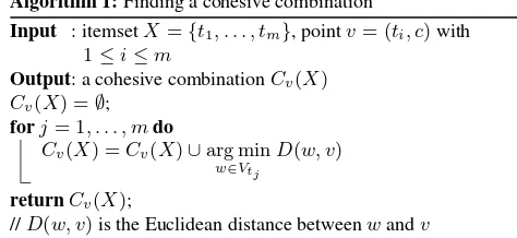
Intuitively, points that occur near to each other are more likely to produce the smallestM axD(V)than those far apart. There-fore, rather than looking at all possible combinations, we limit our search to a selection of points. We propose an algorithm (as described in Algorithm 1) to first find a cohesive combination Cv(X)containing a pointv= (ti, c)(cis then-dimensional
co-ordinate of the point andi∈ {1, . . . , m}) and occurrences of all other items ofXnearest tov.
Algorithm 1:Finding a cohesive combination
Input : itemsetX ={t1, . . . , tm}, pointv= (ti, c)with 1≤i≤m
Output: a cohesive combinationCv(X)
1 Cv(X) =∅;
2 forj= 1, . . . , mdo
3 Cv(X) =Cv(X)∪arg min w∈Vtj
D(w, v)
4 returnCv(X);
//D(w, v)is the Euclidean distance betweenwandv
Lemma 1. Given itemsetX ={t1, . . . , tm}, and a pointv = (ti, c), with1≤i≤m,M axD(Cv(X))found by Algorithm 1,
can never be more than twice as large asdv(X).
Proof. Given a data pointv, Algorithm 1 will get a combination Cv(X)enclosingvand the occurrences of all other items inX
closest tov. Since we know that there exists a combinationV withM axD(V) =dv(X), we can conclude that, for any item
tjinX, the maximal distance fromvto the nearest occurrence of
tjcannot be larger thandv(X). It follows thatM axD(Cv(X))
is at most2×dv(X).
Based on Lemma 1, we approximate the process of computing the cohesive distance ofXas follows:
1. select itemt1fromX={t1, . . . , tm}(items are sorted by
fre-quency in descending order since this computes a more accurate average (Zhou et al., 2015)), and for each pointvj ∈Vt1, j = 1,2, . . . ,|Vt1|, we findCvj(X)as described in Algorithm 1 and getM axD(Cvj(X)).
2. we denote the cohesive distance ofXin a structureSas
D(X) = P
vj∈Vt1M axD(Cvj(X))
|Vt1|
. (1)
There are only|Vt1|combinations to find in a structureS, much
fewer than if we tried to check all combinations for each occur-rence of t1 in S, resulting in a considerable reduction in time
complexity.
However, this procedure inevitably results in approximation er-rors. For example, as illustrated in Figure 3, assume we are evalu-ating itemsetabc, and we picked itemaas the first item. We look for the nearestband the nearestc, and findb1andc1, which are
closer toa1thanb2andc2, respectively, resulting in the dashed
line whose length is M axD(a1b1c1). However, the smallest
M axD(V), whereV containsa,bandc, is much smaller, and is depicted using a solid line, i.e., da1(abc) =length ofa1c2.
In practice, such cases are rarely encountered. Therefore, this approximate method is capable of producing reasonably accurate results.
Figure 3. An example of an approximation error.
3.2 Co-location Pattern
Given a maximum cohesive distance thresholdmax dis,X is a
co-location patternor acohesive itemsetifD(X)≤max dis. In this case, we say thatX is cohesive. Note that the smaller the distanceD(X)the higher the cohesion ofX. A single item will always be cohesive since the cohesive distance of a singleton is always equal to 0.
The constraint of this approximate method gives a guarantee that when the first item from a co-location pattern is encountered, the remainder of the set is likely to be found nearby.
4. COLOCATION PATTERN MINING ALGORITHM
In this section we present an algorithm for mining co-location patterns in a single structure containing a number of multidimen-sional points.
4.1 Search For Itemsets
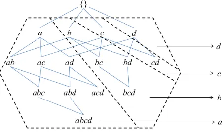
Figure 4. Depth-first search.
4.2 Pruning
The cohesive distance of an itemset is not a monotonic measure. In other words, it is possible for the cohesive distance of a smaller itemset to be greater than the cohesive radius of one of its super-sets. For example,D(bc)may turn out to be larger thanD(abc) as we are computing the maximum distances around different data points. As shown in Figure 5,D(bc) > D(abc)since the average ofM axD(b1c1)andM axD(b2c1)is much larger than
M axD(a1b1c2).
Figure 5. An example resulting in a larger itemset having a smaller cohesive distance.
As a result, we are unable to use the standard itemset mining pruning techniques that rely on the quality measure (typically fre-quency) being anti-monotonic. However, we here present alterna-tive pruning techniques that are applicable in our method, which allow us to develop an efficient algorithm for the cohesion based co-location pattern mining task.
Although the cohesive distance of an itemset is not monotonic, we can still use its properties for pruning certain candidates from the search space. Our pruning method is based on the following lemma:
Lemma 2. Assume itemsetXis a subset of itemsetY, and all the items ofXandY are sorted by the same order. If they share the same first item, thenD(X)≤D(Y).
Proof. Denote the first item inXandY witht. Given an occur-rencevioft, our method finds a cohesive combinationCvi(X) for itemsetX. Clearly,M axD(Cvi(Y))cannot be smaller than
M axD(Cvi(X))if we insist thatCvi(Y)also contains the near-est occurrences of all items inY \X. Our method finds such combinationsCvi(Y)for each occurrence oft, and then com-putes the average value ofM axD(Cvi(Y)). Given thatXand
Y share the first itemt, the number of such combinations will be the same forX andY, and eachM axD(Cvi(Y))will be at
least as large as the correspondingM axD(Cvi(X)). Therefore,
D(Y)will be at least as large asD(X).
Therefore, we can prune itemsets which are not cohesive when we generate itemsets in the depth-first way as shown in Figure 4.
4.3 Algorithm
After choosing the way of enumerating the itemsets and the prun-ing method, we design the algorithm to generate all co-location patterns. Our algorithm generates all co-location patterns in two steps. In the first step, we use the depth-first search method to generate candidate itemsets. In the second step, we determine which of the itemsets are actually spatially cohesive and utilise the observations above to prune the itemsets that cannot be cohe-sive.
Letn-itemset denote an itemset of sizen. LetFn denote the
set ofn-itemsets andTn be the set of cohesiven-itemsets.
Al-gorithms 2 and 3 show the process of generating all co-location patterns. Frequency constraintsmin freandmax frecan be used to filter out items which are not interesting, due to being either too frequent or not frequent enough. For example, in ourcitydataset (see Section 5 for details), there are trash cans on every corner, and patterns including trash cans are therefore of little value to the user. Optional parameters,min sizeandmax size, can be used to limit the output only to co-location patterns with a size bigger than or equal tomin sizeand smaller than or equal tomax size.
Algorithm 2:GENERATINGCOLOCATIONPATTERNS. An algo-rithm for generating all co-location patterns in a structure. Input : structureS, frequency constraintsmin fre,max fre,
maximum cohesive distance thresholdmax dis, pattern size constraintsmin size,max size.
Output: all co-location patternsT.
1 F1={t|t∈I,min fre≤F re(t)≤max fre};
2 if1≥min sizethen 3 T1=F1;
4 sort(F1);
5 Depth-First-Search(F1);
6 T =STi;
7 returnT;
Algorithm 3:Depth-First-Search(Q)
Input : a set of itemsetsQsharing all but the last item 1 foreachαiinQdo
2 Fi=∅;
3 foreachαjinQ, withj > ido
4 X=αi+last item(αj);
5 if|X| ≤max sizeandD(X)≤max disthen
6 Fi=Fi∪ {X};
7 if|X| ≥min sizethen 8 T|X|=T|X|∪ {X};
9 Depth-First-Search(Fi);
In Algorithm 2, lines 1-3 count the frequency of all the items to determine the cohesive 1-itemsets. Line 4 sorts the items inF1by
descending frequency. Line 5 calls Algorithm 3 to get cohesive n-itemsets (max size≥n≥2). Finally, we get the complete set of co-location patternsT(lines 6-7).
In Algorithm 3, given any twon-itemsetsαiandαjthat share
of lengthn+ 1by adding the last item inαjtoαi(line 4). In
lines 5-6, we prune the candidates that cannot be cohesive by the properties. Then in lines 7-8, we store the cohesive itemsets into Tn.
5. EXPERIMENTS
We compared our pattern miner, calledCoDis, with the method proposed by Huang et al. (Huang et al., 2004) (which we call
LW-prevsince the method mines prevalent patterns by a “level-wise” approach) and the1-descendmethod proposed by Zhou et al. (Zhou et al., 2015). We implemented the methods in Java and all experiments were performed on a 2.90GHz Ubuntu machine with 2GB memory.
All the presented methods use some sort of a distance threshold dt, i.e., the maximum cohesive distance thresholdmax disfor our methodCoDis, the neighbourhood thresholdntforLW-prev, and the maximum cohesive radius thresholdmax radfor1-descend. In all experiments, we keepdt = nt = max rad = max dis
2 to
make a fair comparison.
Thecitydataset we used is one 2-dimensional structure obtained from the open data of the city of Antwerp in Belgium1. We first downloaded the datasets containing coordinates of different in-frastructure objects with locations, e.g., schools, kindergartens, city offices, playgrounds, cultural institutions, public toilets, re-cycling centres, trash cans, waste rere-cycling bins, glass rere-cycling bins, hospitals, and so on. We expanded the dataset by adding some data about the city neighbourhoods2from 2009, i.e., aver-age aver-age, percentaver-age of immigrant population and averaver-age income per person, all of which are numeric attributes. Therefore, we first discretised such numbers into different levels based on the information given on the website and used the coordinate of the centroid of a neighbourhood as its location. Table 1 shows a few examples of the items generated in this way. Finally, we merged the datasets together, and thus obtained a 2-dimensional structure containing 6424 points carrying 33 different items.
Attribute Item Example Meaning
average age age42-45 the average age in the neighbourhood is
be-Table 1. Examples of items generated from the demographic data.
5.1 Analysis of Discovered Patterns
The most cohesive itemsets turned out to be singletons, which was to be expected, since singletons always have a cohesive ra-dius equal to 0. To obtain more meaningful results, we decided to look only for itemsets of size 2 or higher. Therefore, for all methods,min sizewas set to 2 andmax sizeunlimited. We fur-ther found that most of the cohesive itemsets contained trash cans,
1
http://opendata.antwerpen.be/ 2
http://www.antwerpen.buurtmonitor.be/
glass recycling bins or recycling bins, which was not surprising, as there were 3750 trash cans, 551 glass recycling bins and 344 recycling bins in the dataset, making their frequencies a lot larger than that of any other item. As a result, we disregarded these items by settingmax freto 340. We setmin freto 5 to prevent items that hardly ever occur from becoming part of a pattern.
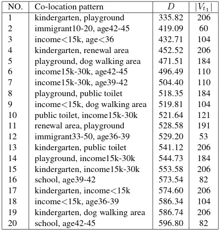
We first ranCoDiswithmax dis= 600 metres, discovering the 20 patterns shown in Table 2 in 0.122 seconds. D means the cohesive radius of the discovered co-location pattern and|Vt1|is
the frequency of the first item of the pattern. Concrete examples of interesting patterns included the fact that the higher the average age, the higher the average income (patterns 3,6,7 and 18) in a neighbourhood, or that given a kindergarten, there is likely to be a playground nearby (pattern 1). From patterns 2 and 12, we can see that immigrants are likely to be young people. Compare to the patterns mined by1-descendwithmax rad= 300 metres, we find thatCoDisgets the same patterns.
NO. Co-location pattern D |Vt1|
1 kindergarten, playground 335.82 206 2 immigrant10-20, age42-45 419.09 60 3 income<15k, age<36 432.71 104 4 kindergarten, renewal area 452.52 206 5 playground, dog walking area 471.51 184 6 income15k-30k, age42-45 496.49 110 7 income15k-30k, age39-42 504.40 110 8 playground, public toilet 518.35 184 9 income<15k, dog walking area 519.81 104 10 public toilet, income15k-30k 521.64 121 11 renewal area, playground 528.58 191 12 immigrant33-50, age36-39 529.20 53 13 kindergarten, public toilet 541.12 206 14 playground, income15k-30k 544.73 184 15 kindergarten, income15k-30k 553.58 206
16 school, age39-42 573.54 82
17 kindergarten, income<15k 574.60 206 18 income<15k, age36-39 586.34 104 19 kindergarten, dog walking area 586.74 206
20 school, age42-45 596.80 82
Table 2. Co-location patterns found byCoDis.
5.2 Impact of Distance Threshold on Runtime
Figure 6 shows the runtimes of the methods with various distance thresholds where other parameters are kept the same as before. We ranLW-prevwith the prevalence threshold set to 0.1. The re-sults show that, as the distance threshold increases, the runtimes of all methods increase. This is because a larger distance thre-shold will increase the number of candidate patterns that need to be processed. We find that the runtime ofLW-previncreases too fast while the runtimes of other methods are acceptable. It can be noted thatLW-prevruns out of memory when the distance threshold is 800 since the process of identifying prevalent co-location patterns needs more memory than the computations re-quired by our algorithms. CoDisappears to be the most scalable method, and the runtime ofCoDisis almost half of the runtime of1-descend.
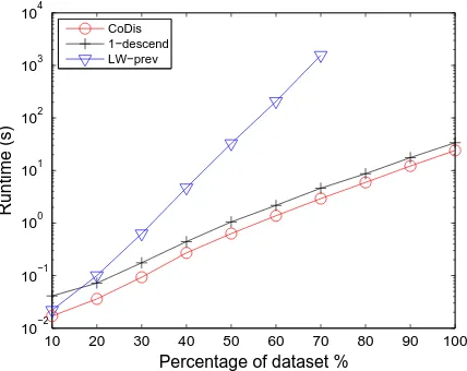
5.3 Impact of Structure Size on Runtime
Figure 7 shows the runtimes of the methods with respect to dif-ferent number of points (varying from 10% to 100% of the whole structure). In this experiment we use the whole structure without settingmin freandmax frefor the items. We setmin sizeto 2,
200 300 400 500 600 700 800 10−1
100 101 102 103 104
Distance threshold
Runtime (s)
CoDis 1−descend LW−prev
Figure 6. Impact of the distance threshold on the runtime.
10 20 30 40 50 60 70 80 90 100
10−2 10−1 100 101 102 103 104
Percentage of dataset %
Runtime (s)
CoDis 1−descend LW−prev
Figure 7. Impact of the structure size on the runtime.
all methods. We ran LW-prev with the prevalence threshold set to 0.1. We repeated the experiment ten times, using ten different random permutations of the data points. The reported runtimes are therefore averages of the ten different runs. For all methods, the runtime grows with increasing number of points. The LW-prevmethod seems to be prohibitive, whileCoDisis the fastest. Comparing the resulting patterns, we find thatCoDisperforms comparably in terms of accuracy while achieving much quicker runtimes.
6. CONCLUSION
The abundance of spatial data provides exciting opportunities for new research directions but also demands caution in using these data. Handling the very large volume and understanding complex structure in spatial data are two major challenges for spatial data mining, which demand both efficient computational algorithms to mine large datasets for interesting patterns.
In this paper, we have presented a methodCoDisto efficiently mine co-location patterns in multidimensional spatial data. We applied the method to find spatially cohesive patterns from the spatial data of a city and the resulting patterns demonstrated the efficiency and intuitiveness of the proposed method. Through experimental evaluation, we confirmed thatCoDisimprove the efficiency of1-descendby avoiding to find the smallest enclosing
ball of points. CoDisgives a guarantee that when the first item from a co-location pattern is encountered, the remainder of the set will be found nearby.
REFERENCES
Agrawal, R. and Srikant, R., 1994. Fast algorithms for mining association rules. In: VLDB’94, Morgan Kaufmann Publishers, pp. 487–499.
Barua, S. and Sander, J., 2014. Mining statistically significant co-location and segregation patterns. IEEE Transactions on Knowl-edge and Data Engineering26(5), pp. 1185–1199.
Huang, Y., Pei, J. and Xiong, H., 2006. Mining co-location pat-terns with rare events from spatial data sets. Geoinformatica
10(3), pp. 239–260.
Huang, Y., Shekhar, S. and Xiong, H., 2004. Discovering colocation patterns from spatial data sets: a general approach.
IEEE Transactions on Knowledge and Data Engineering16(12), pp. 1472–1485.
Koperski, K. and Han, J., 1995. Discovery of spatial associa-tion rules in geographic informaassocia-tion databases. In: Advances in spatial databases, Springer, pp. 47–66.
Morimoto, Y., 2001. Mining frequent neighboring class sets in spatial databases. In: Proceedings of the seventh ACM SIGKDD international conference on Knowledge discovery and data min-ing, ACM, pp. 353–358.
Shekhar, S. and Huang, Y., 2001. Discovering spatial co-location patterns: A summary of results. In: Advances in Spatial and Temporal Databases, Springer, pp. 236–256.
Xiao, X., Xie, X., Luo, Q. and Ma, W.-Y., 2008. Density based co-location pattern discovery. In:Proceedings of the 16th ACM SIGSPATIAL international conference on Advances in geo-graphic information systems, ACM, p. 29.
Yoo, J. S. and Shekhar, S., 2006. A joinless approach for mining spatial colocation patterns.IEEE Transactions on Knowledge and Data Engineering18(10), pp. 1323–1337.
Zhang, X., Mamoulis, N., Cheung, D. W. and Shou, Y., 2004. Fast mining of spatial collocations. In:Proceedings of the tenth ACM SIGKDD international conference on Knowledge discovery and data mining, ACM, pp. 384–393.
Zhou, C., Cule, B. and Goethals, B., 2015. Cohesion based co-location pattern mining. In: Proceedings of the International Conference on Data Science and Advanced Analytics (DSAA).
ACKNOWLEDGEMENTS