AUTOMATIC CLASSIFICATION OF COARSE DENSITY LIDAR DATA IN URBAN AREA
H. M. Badawy a, *, A. Moussaa, N. El-sheimya
a Department of Geomatics Engineering, University of Calgary, 2500 University Dr. NW, Calgary, AB T2N 1N4, Canada (hmmohamm, amelsaye,elsheimy)@ucalgary.ca
Commission V Close-Range Imaging, Analysis and Applications
KEY WORDS: LIDAR, Vehicle, Classification, Airborne, Urban, PCA, NDSM, DTM
ABSTRACT:
The classification of different objects in the urban area using airborne LIDAR point clouds is a challenging problem especially with low density data. This problem is even more complicated if RGB information is not available with the point clouds. The aim of this paper is to present a framework for the classification of the low density LIDAR data in urban area with the objective to identify buildings, vehicles, trees and roads, without the use of RGB information. The approach is based on several steps, from the extraction of above the ground objects, classification using PCA, computing the NDSM and intensity analysis, for which a correction strategy
was developed. The airborne LIDAR data used to test the research framework are of low density (1.41pts/m2) and were taken over an urban area in San Diego, California, USA. The results showed that the proposed framework is efficient and robust for the classification of objects.
* Corresponding author.
1. INTRODUCTION
The problem of classification of objects from low density LIDAR point cloud in urban area is challenging, especially when there is no RGB information associated with the point cloud. The aim of this paper is to fully classify objects in the urban areas such as buildings, vehicles, roads and green regions (trees and grass).
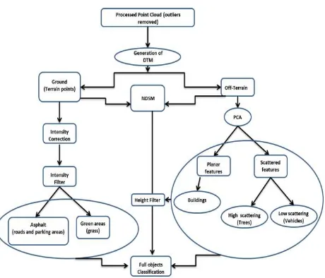
We build a framework in order to approach full classification of these objects. The framework has several steps starting with generating a Digital Terrain Model (DTM) for the point cloud in order to isolate terrain points from off-terrain points. The second step uses the Principal Component Analysis (PCA) as a segmentation tool for the off-terrain point cloud. The PCA segmentation technique is useful to discriminate buildings (planer points) from trees and vehicles (scattered points). However, some buildings with roofs containing pipelines or windows will lead to a scattered LIDAR points. The scattered points above a certain height could be eliminated with the use of Normalized Digital Surface Model (NDSM) which is the third step in the classification framework. NDSM is used to filter objects with heights above a certain threshold. The last step in the framework is to use the corrected LIDAR points’ intensity as a filter discriminating the grass area from asphalt roads and parking areas.
In the following section will provide more details of the framework. In the third section, the test data and their characteristics are introduced. The fourth section includes the discussion and analysis of the obtained results.
2. CLASSIFICATION FRAMEWORK
Figure (1) shows the general steps of, the proposed classification framework which includes: DTM generation, PCA, NDSM and intensity filters as will be discussed in the following subsection.
Figure 1. The general classification framework of airborne LIDAR data
2.1 Generation of DTM
There are many filtration methods to obtain the DTM from point cloud. Among these are morphological filters, surface based filers and segment based filters (Vosselman & Maas, 2010). In this paper we implmented moropological filters as a tool of generation the DTM following the work done by (Vosselman, 2000) and (Sithole, 2001). (Vosselman, 2000) used the difference in height h over the euclidian distance d to filter data. In order to compare the points within a specified distance, the points had to be organized in a Delaunay triangulation. A height threshold was chosen so that the difference in height between two points with a distance d The International Archives of the Photogrammetry, Remote Sensing and Spatial Information Sciences, Volume XL-5, 2014
should not exceed 0.3d. (Sithole, 2001) made some between points and therefore his method, with its computational complexities, is not needed in urban areas where gentle slopes occur.
In this paper, the DTM is generated based on the minimum height in the neighborhood. We first organize the point cloud in a 3-dimensional kD-tree. Afterwards we search for the local minima in each neighborhood. The kD-tree search algorithm not only is useful for the DTM generation, but it is also used in the PCA segmentation technique.
In the proposed algorithm, we find the minimum height of each neighborhood then compare it with all the points in the neighborhood. If the differencehbetween the minimum height and the height of a point in the neighborhood is lower than a robust results, the radius of the kD- tree search had to be chosen as wide as possible so as to combine points of the ground with the neighborhood of wide area roofs.
2.2 PCA of the points in the neighbourhood (i.e. planar or scattered). For example, if the search radius was too large (e.g. 20 meters), LIDAR points from trees, vehicles and buildings might be included in the same neighbourhood, consequently, the decision that a certain neighbourhood has a planar or scattered behaviour might not be accurate. On the other hand, if the search radius was chosen to be too small (e.g. 1 meter) the number of neighbourhood points might not be enough to detect their covariance behaviour especially with low density point
cloud (i.e. 1.41pts/m2). We chose a search radius of 3 meters in order to cover single trees or single vehicles. The 33 symmetric covariance matrixCvof each neighbourhood
associated with each point in the point cloud is computed as:
The geometry of the distribution of the points can be identified from the eigenvalues of the covariance matrix. Basically, if one of the eigenvalues is larger than the two other eigenvalues, it means that the LIDAR points are linearly distributed in the direction of the vector associated with that eigenvalue. If two of the eigenvalues are almost equal but larger than the third eigenvalue, this means that the LIDAR points are distributed in the plane containing the two vectors associated with these two eigenvalues. If the case is that all the eigenvalues are almost equal. This means that the LIDAR points are distributed in a scattered form in a three dimensional space.
Then the following geometric classifications, which are based on the properties of the eigenvalues discussed above, are used to make a decision on the behaviour of the points in a neighbourhood [for more details, see (Carlberg, et al. 2009) and (Shi and Zakhor 2011)]: vehicles, we assume that if 3is below a certain threshold value then the scattered laser points are reflected from vehicles. The fact that the laser points reflected from vehicles have low scattering characteristics than the trees is due to the difference in geometrical shapes between trees and vehicles.
2.3 Obtaining the NDSM
Although the points reflected from buildings should have a planar behaviour, some points might be scattered due to pipelines or glassy windows attached to their roofs. This leads to confusion in discriminating some of the points reflected from buildings from those reflected from trees or vehicles. On the other hand, discrimination between vehicles and trees could not be guaranteed to be 100 % accurate if we only rely on the scattering properties, especially when the 3D-tree search radius is set to a possibly large value.
In order to tackle these problems we use the NDSM to further identify objects based on their absolute height.
In order to determine the off-terrain objects’ heights above the ground (DTM), the NDSM is produced by subtracting the DTM height from the off-terrain objects’ heights (Ekhtari, et al. 2009). In order to compute the NDSM we use the 2D-tree search algorithm to find the closest DTM neighbourhood of the off-terrain points and subtract the height of their minima from order to solve this issue, instead of searching for neighbouring points in a specified radius, we use the k-nearest points’ algorithm to search for a specific number of nearest DTM points close to the off-terrain points. It should be noticed that if an off-terrain point was incorrectly identified as a terrain point, that point would generate errors in the NDSM computation. In order to avoid this, we find the point with minimum height of The International Archives of the Photogrammetry, Remote Sensing and Spatial Information Sciences, Volume XL-5, 2014
the DTM k-nearest points associated with the off-terrain point of interest, and then we subtract the height of both points.
NDSM {hp min hpj :pDTMj Nj C} applications beside objects classification (such as strip adjustment, forestry, etc...). Several factors influence the received laser intensity (power), for example:
a) Spherical loss. b) Topographic effects. c) Atmospheric attenuation.
Hence the intensity recorded by the laser scanner is not reliable for the process object classification. Therefore, a number of corrections must be made to the intensity values in order to benefit from it in object classification.
(Höfle and Pfeifer 2007) introduced two approaches for the recorded intensity correction. The first approach is called data-driven correction. This approachuses predefined homogeneous areas for the estimation of the best parameters for a global correction function that takes into account all range-dependent influences (using least-squares). The second approach is called the model driven correction. In this approach each recorded intensity value is corrected independently based on the physical principle of LIDAR systems.
In this paper, we used the model driven correction since we don’t have a predefined area associated with the data that we have.
The formula given by (Höfle & Pfeifer, 2007) is:
between the surface normal and the incoming laser shot ray, I is the recorded intensity, Rs is a user-defined standard range and a is the atmospheric attenuation coefficient measured in dB/km.
In this paper we use intensity as a mean of discrimination between grass and asphalt regions (including roads and parking areas). The reason why we use intensity with the DTM points is that DTM points are mostly flat in urban areas, and therefore can’t be segmented based on the PCA technique. On the other hand, PCA and NDSM are used efficiently with the off-terrain objects identification (i.e. no need for further processing regarding their intensity values).
.
3. RESULTS ANALYSIS AND DISCUSSION
3.1 Test Data
The test data was obtained from the OpenTopography portal on the internet (http://www.opentopography.org). The data were
collected in 2005 over the city of San Diego, California, USA.
The point cloud density is1.41pts/m2. The data were collected over an area of 1,190.00 km. A subset of the data with an area of (850m670m) was used as a test data. The test data were used such that it is full of urban objects such as buildings, vehicles and trees.
3.2 Visual assessment of the results
Figure (2) shows an image of the reference test area (ground truth). The image was taken from Google Earth, version (7.1.2.2041). The image date is August 26th, 2005.
Figure 2. Ground truth image of the test area.
It should be mentioned here that there might be some differences related to the number of vehicles and their shapes in the ground truth image and the processed LIDAR Data. This is mainly because there is a temporal difference between the image taken for the area and the LIDAR data collection.
Figures (3) and (4) show the extracted DTM and off-terrain points, respectively. A comparison between the ground truth in Figure (2) and both DTM and off-terrain images shows that the filter used for the generation of DTM is efficient and robust especially with wide roofs.
After the extraction of the DTM points, the intensity filter was used to discriminate the asphalt regions from the grass.
In order to filter the data using intensity values, we used the histogram to gain information about the distribution of the intensity values and hence the distribution of grass and asphalt regions. Figure (5) shows the histogram of the intensity values of the DTM points. There are two spike peaks at the intensity values of 255 and 0. Other peaks are close to the peak at intensity of 0 values. It is expected that the grass has a higher return intensity than that of the asphalt regions. It is obvious then from the histogram that the intensity of the grass has a peak around the value 255 whereas the other peaks are the associated with the asphalt regions.
Figure 3. The extracted DTM points.
Figure 4. The extracted off-terrain points.
This histogram is used to detect the intensity threshold value at which the DTM is either considered as grass or asphalt.
Figure 5. Histogram of the intensity values of the DTM points.
Based on the intensity filter, the result of classification of DTM points is shown in Figure (6). The points coloured black are the asphalt regions which is either roads or parking areas and the points coloured green are grass.
Figure 6. Classification of DTM points into grass and asphalted regions.
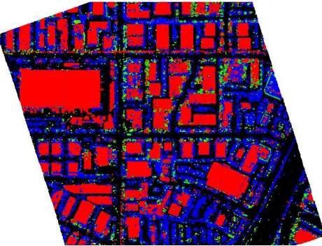
Figure (7) shows the full objects classification of the test area, where buildings were assigned the red colour, vehicles were assigned the blue colours, the black colour is assigned to the asphalt regions and the green colour for the green regions ( trees and grass).
Figure 7. Full classification of the coarse LIDAR point cloud.
3.3 Classification quality assessment
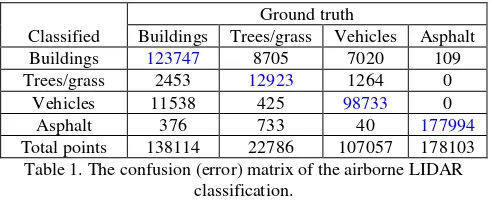
In order to statistically assess the results of the proposed classification framework, we compare the final classification results with the ground truth. The result of this comparison is a confusion (error) matrix and its associated Cohen’s kappa coefficient. Table (1) shows the confusion matrix. The total number of points is given with the number of points correctly or incorrectly classified.
Classified
Ground truth
Buildings Trees/grass Vehicles Asphalt
Buildings 123747 8705 7020 109
Trees/grass 2453 12923 1264 0
Vehicles 11538 425 98733 0
Asphalt 376 733 40 177994
Total points 138114 22786 107057 178103 Table 1. The confusion (error) matrix of the airborne LIDAR
classification.
The confusion (error) matrix describes the amount of agreement between the ground truth and the classified objects. The diagonal of the matrix describes the agreement between the ground truth of an object and its classification. Their sum is the overall proportion of observed agreement:
P0
pii (7)The off-diagonal elements describe the agreement that happened by chance between an object and another object. The sum of the off-diagonal elements is called chance-expected agreement:
j
j i
i
e p p
P
(8)
The Cohen kappa coefficient associated with the confusion matrix is then given by:
e e
P P P
1
0
(9)
This coefficient is a measure of the agreement between classification and ground truth. It takes on a value of 1 with perfect agreement. It has a value close to 0 if the agreement is expected to be by chance (i.e. incorrect classification). Values of above 0.75 indicate very good to excellent agreement [for more details, see (Monserud & Leemans, 1992) and (Cohen, 1960)].
The value of Cohen kappa coefficient associated with the confusion matrix in Table (1) is0.8925, which implies an excellent agreement between the classification and the ground truth.
4. CONCLUSION
This paper presents a framework for the classification of low density airborne LIDAR data. The framework is based on PCA, generation of DTM and NDSM and the use of intensity filter. The visual and statistical assessments of the results proved an efficient and robust automatic classification results in the urban areas. Test results shows that although the LIDAR data was of low density, there is an excellent agreement between the classified objects and the ground truth. This can be concluded from the value of Cohen’s kappa coefficient. That proves that the classification framework was successful.
ACKNOWLEDGEMENTS
This work was supported in part by research funds from TECTERRA Commercialization and Research Centre, and the Natural Science and Engineering Research Council of Canada (NSERC) to Dr Naser El-Sheimy.
This material is based on data provided by the OpenTopography Facility with support from the National Science Foundation under NSF Award Numbers 0930731 & 0930643.
REFERENCES
Carlberg, M., Gao, P., Chen, G., & Zakhor, A. (2009). classifying urban landscape in aerial lidar using 3d shape analysis. 16th IEEE International Conference on Image Processing (ICIP). Cairo: IEEE.
Cohen, J. (1960). A Coefficient of Agreement for Nominal Scales. Educational and Psychological Measurement, 20(1), 37-46.
Ekhtari, N., Zoej, M. J., Sahebi, M. R., & Mohammadzadeh , A. (2009). Automatic building extraction from LIDAR digital elevation models and WorldView imagery. Journal of Applied Remote Sensing, 3(1), 1-12.
Höfle, B., & Pfeifer, N. (2007). Correction of laser scanning intensity data: Data and model-driven approaches. ISPRS Journal of Photogrammetry & Remote Sensing, 62, 415-433.
Monserud, R. A., & Leemans, R. (1992). Comparing global vegitation maps with the Kappa statistics. Ecological modelling, 62, 275-293.
Shi, x., & Zakhor, A. (2011). FAST APPROXIMATION FOR GEOMETRIC CLASSIFICATION OF LIDAR RETURNS. 18th IEEE International Conference on image processing. Brussels: IEEE.
Sithole, G. (2001). FILTERING OF LASER ALTIMETRY DATA USING A SLOPE ADAPTIVE FILTER. International Archives of Photogrammetry and Remote Sensing, 34(3/W4), 22-24.
Vosselman, G. (2000). SLOPE BASED FILTERING OF LASER ALTIMETRY DATA. International Archive of photogrammetry, remote sensing, 33(3B), 935-942.
Vosselman, G., & Maas, H.-G. (2010). Airborne and Terrestrial laser scanner. Caithness, Scotland, UK: whittles Publishing. The International Archives of the Photogrammetry, Remote Sensing and Spatial Information Sciences, Volume XL-5, 2014