www.elsevier.com/locate/econedurev
Efficiency and costs in education: year-round versus
traditional schedules
Nasser Daneshvary
a,*, Terrence M. Clauretie
baDepartment of Economics, University of Nevada, Las Vegas, 4505 Maryland Parkway, Las Vegas, NV 89154-6005, USA bDepartment of Finance, University of Nevada, Las Vegas, 4505 Maryland Parkway, Las Vegas, NV 89154-6005, USA
Received 1 May 1997; accepted 9 November 1999
Abstract
This study explores the cost savings (efficiency) of a year-round schedule versus a traditional 9-month schedule for schools in Clark County, Nevada. Unlike many previous studies, the cost of real estate capital is included in the estimated cost functions. The sample includes 115 elementary schools, 26 with a year-round schedule, and the study finds that this schedule not only produces efficiencies in the cost of capital area but also in other areas such as operations. These efficiencies are evident after taking into account the usual average daily attendance, test performance scores, and socioeconomic variables that are customarily used in such studies. The existence and size of efficiencies discovered in this study have implications for those school districts that face a rapidly growing student population.2001 Elsevier Science Ltd. All rights reserved.
Keywords: Efficiency; Education; Year-round
1. Introduction
Numerous papers have been written concerning cost or production efficiency in education. Some papers focus on cost minimization subject to output or performance (Barrow, 1991; Jimenez, 1986; Watt, 1980) or on output maximization subject to cost constraints (Deller & Rud-nicki, 1993; Callan & Santerre, 1990; Hanushek, 1986; Levin, 1974). One issue explored in these papers is the comparative efficiency between schools in the same jur-isdiction (county, state). The stated purpose of such stud-ies is to determine the degree to which some schools may operate less efficiently than others or less efficiently than their own potential. Other papers explore economies of size (Duncombe, Miner, & Ruggiero, 1995; Kumar, 1983; Kenny, 1982; Fox, 1981). These papers explore
* Corresponding author. Tel.: +1-702-895-3362; fax: + 1-702-895-4090.
E-mail address: [email protected] (N. Daneshvary).
0272-7757/01/$ - see front matter2001 Elsevier Science Ltd. All rights reserved. PII: S 0 2 7 2 - 7 7 5 7 ( 0 0 ) 0 0 0 1 0 - 8
the (reduced) per pupil costs which result from enlarged school size. Callan and Santerre (1990), for example, conclude that some savings may derive either from con-solidation (merging primary and secondary school districts) or from a more optimal use of real estate capi-tal. Their results suggest that the typical school district overemploys capital in the short run. The short-run excess capacity of real estate capital probably flows from the indivisibility of this input.
infor-mation on the physical size of the schools is seldom reported by school district officials. One of the few pap-ers to include a cost of capital is Callan and Santerre (1990). Yet even here the authors employ a proxy;
expenditures on land, buildings, and debt service,
because the value of the real estate capital was unavail-able for their study.
Although real estate capital can be utilized more efficiently by increasing the number of pupils as the excess space allows, another method by which it can be made more divisible, and thus more efficient, is through the use of flexible scheduling such as year-round instruc-tion. An extended school schedule allows a more inten-sive use of the real estate.
The purpose of this study is to estimate the impact of a year-round schedule on the cost structure of elementary schools in southern Nevada, a cost structure that includes the cost of real estate capital. This paper makes two con-tributions: it includes real estate capital as a cost element in an economy of size study and it explores the effect of implementing a year-round schedule on all costs, including administrative, instruction, operation, and stud-ent support.
The following section discusses the year-round sched-ule. Section 3 presents the model and data. The fourth section discusses the empirical results and the final sec-tion is the conclusion.
2. The year-round schedule in a model of education costs
The “traditional” school term for kindergarten through grade 12 refers to a term that is approximately 9 months long with a 3-month break during the summer months. The term year-round school refers to a schedule whereby a particular student attends the same number of total days as with the traditional schedule but reallocates the long summer vacation to shorter periods spread out over the entire year. The shorter vacation period does not rep-resent a period for which the capital is not used, how-ever, as students attend school in tracks that are stag-gered. Geisert (1990) claims that the most popular year-round schedule is the 45–15 model where students attend 9 weeks of classes followed by 3 weeks of vacation. He reported that year-round schools have been implemented in areas where student overcrowding is a concern and where there is a lack of funding for new school construc-tion.
The year-round schedule may also improve the quality of education. Geisert (1990) indicates that there is an increase in student motivation and less absenteeism with this schedule. Finally, he claims that teachers may prefer this schedule because there are more frequent but shorter vacations. This leads to less burnout for teachers, more motivated students, and less time spent reviewing
material from the previous term. Woo (1987) reported that while 38 percent of respondents (with children) to a survey favored the year-round schedule, 51 percent did not. However, of those respondents with children in a year-round school this schedule was favored by a 51 per-cent to 44 perper-cent margin.
2.1. Description of the Clark County, Nevada, year-round schedule
As indicated, a year-round schedule makes greater use of the real estate capital by eliminating the long summer term and by operating in “shifts” or “tracks.” With a 12-week-on and 3-week-off schedule approximately 25 percent more students can utilize the real estate facilities than with a traditional 9-month schedule. An example of a year-round track schedule is shown in Table 1. At each year-round school there are four or five different tracks. Each student is placed in a given track and, as can be seen in Table 1, breaks occur in different places for each of the tracks. For a given track both teachers and students are off at the same break time (except for special edu-cation students who, by law, must attend school on a full-time year-round schedule and are taught by teachers on a special 12-month contract). There are no greater contact hours for teachers in year-round schools than for traditional schedule schools. The staggered breaks allow for continued occupancy of the school facility. It is this continuity of use that is expected to lead to savings in the cost of real estate capital. One would expect that if the facilities are used more intensively in a year-round school then utility and maintenance costs may increase, offsetting potential savings in other areas. Although there
Table 1
1997–98 school calendar at Mary Doe Elementary School
Track 1 calendar
September 25–December 19 Trimester 1 January 5–January 27 Break January 28–April 24 Trimester 2 April 27–May 22 Break May 26–August 13 Trimester 3
August 13 End of school year
Track 2 calendar
August 25–September 23 Trimester 1 September 24–October 24 Break
October 27–December 19 Trimester 1 (cont.) January 5–January 27 Trimester 2 January 28–February 24 Break
February 25–April 24 Trimester 2 (cont.) April 27–May 22 Trimester 3
May 26–June 16 Break
June 17–August 13 Trimester 3 (cont.)
August 13 End of school year
are no detailed data on these costs, they are included in the general category of operations costs, which is avail-able. Transportation cost data are also unavailable on a school-by-school basis. We suspect, however, that there should be some moderate cost savings if school buses are used more intensively, i.e., not idle during the sum-mer months.
In determining which schools are assigned a year-round schedule, the Clark County District sets several priorities. First, schools are assigned a year-round sched-ule according to their present condition in terms of over-crowded enrollment. Then, elementary schools are assigned a year-round schedule before high schools. Next, a year-round schedule is assigned to those schools where larger future population growth is expected. Finally, on occasion, political considerations come into play. Where parents are well organized and vociferous an unpopular schedule may be avoided. Clark County School District officials report mixed reviews on the year-round schedule. Parents do not universally favor or disfavor this type of schedule but rather take a position determined by their individual family situation. Oppo-sition to one type of schedule or the other is based on a family’s personal employment or vacation schedule. Selection based on this criterion, while unlikely for most households, does raise the possibility that the scheduling variable is endogenous; in other words, that the school costs, performance, and scheduling are determined sim-ultaneously. If it is endogenous, then our coefficient esti-mates in the cost model could be biased. We test for endogeneity of year-round selection, and as discussed in the empirical section, we conclude that this is not a prob-lem.
Nonetheless, where the year-round schedule is implemented, one expects economy in the utilization of fixed resources, particularly real estate capital. The fol-lowing model is intended to capture this effect by look-ing at data for the Clark County, Nevada School District.
3. Model and data
3.1. The theoretical model of cost
Similar to the potential cost savings from school dis-trict consolidation, the potential cost savings from a move to a year-round schedule stems from size or scale economies. The conceptual models on consolidation developed by Fox (1981) and Duncombe et al. (1995) provide a basis for estimating the empirical cost func-tions and identifying potential cost savings resulting from a shift to year-round scheduling.
As with a standard production function, school dis-tricts employ labor, capital, and other inputs to produce a range of educational activities (provision of public services). Modification of such production functions is
needed to account for the distinguishing features of pub-lic services produced by government and the outcomes of interest to citizen-consumers (Hanushek, 1986). Con-sidering the demand characteristics of citizen-consumers, the education production function can be expressed as a process of employing purchased inputs (instruction and real estate) and nonpurchased inputs (student socioecon-omic characteristics) to produce student achievement (Duncombe et al., 1995).
The above modified production framework and pur-chased input prices can be used to derive a cost function which fits education production. The derived cost func-tion is:
TC5f(S,N,F,P) (1) where TC is total cost, S is student achievement (quality of the public service), N is the number of students served by the school, F is family and socioeconomic back-ground or other characteristics of the students, and P is the price of inputs.1 As discussed by Duncombe et al.
(1995), by controlling for student achievement, family and socioeconomic background, and prices, Eq. (1) leads to a clear definition of economies of size. That is, it leads to a clear definition of the relationship between the per pupil cost, TC/N, and the number of students served, N.
3.2. Empirical model, sample, and data
Assuming operation of schools on the downward slop-ing portion of average cost curves, an increase in enrollment, regardless of traditional or year-round sched-uling, may result in an economy of size and lower the average cost. A move to a year-round schedule will increase enrollment and result in an economy of size and lower the average cost. The move to year-round, how-ever, may also shift the average cost curve structure downward, because with the same level of inputs (at least in the case of noninstructional inputs), more “out-put” is obtained.
The sample of schools used in the empirical section of this paper includes observations from both traditional and year-round schools. To avoid confounding the effect of a move to year-round with a purely economy of size effect, which can take place with any type of scheduling,
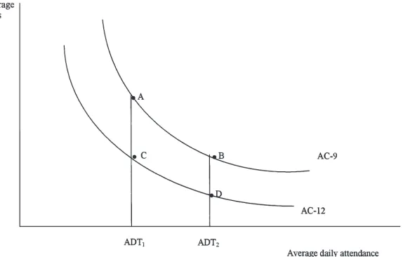
Fig. 1. An illustration of school size change impact on average costs for traditional versus year-round schedules.
we measure the average cost/“output” relationship by constructing an average daily attendance variable (see below). By definition, the average daily attendance vari-able is purged of the effect that a move to year-round scheduling has on the total number of students served (enrollment). In other words, while a move to year-round will increase enrollment, it will not impact the average daily attendance.
The relationship between average cost, average daily attendance, and types of scheduling can be expressed by reference to Fig. 1. For the sake of illustrating, we assume that a move to year-round will lower the average cost at every level of attendance. That is, 9 and AC-12 in Fig. 1 represent the average cost–attendance relationship for 9-month and year-round schools, respectively. An increase of average daily attendance from ADT1to ADT2will result in a movement from A
to B for the 9-month schools and a movement from C to D for the year-round schools. A move from 9-month to year-round, however, may have a structural shift impact and cause a move from AC-9 to AC-12. That is, keeping average daily attendance constant, a move from 9-month to year-round will reduce the average cost from A to C or from B to D.
In order to obtain an accurate and consistent measure of average daily attendance, we used the enrollment and attendance-rate data provided by the school district. Given that a move to year-round schedule increases enrollment by about 25 percent, one could adjust the actual enrollment downward to 75 percent of that figure. However, we were fortunate to have data provided by the Clark County School District that estimates the change in enrollment of each school (year-round and non-year-round) when and if they would be converted to a longer school year. For year-round schools the actual enrollment is adjusted downward to reflect what the
enrollment would be if the school were on a traditional schedule.2
The data were used to estimate the adjustment factor for each year-round school. The adjustment factor was applied to the actual enrollment for each year-round school to obtain adjusted enrollment and then the attend-ance rate was used to calculate average daily attendattend-ance (i.e. average daily attendance=enrollment×adjustment factor×attendance rate). Thus, in the estimated models below, the pure economy of size effect is measured by the coefficient of the average daily attendance variable. The impact of year-round schooling on cost is captured by the inclusion of a dummy variable for year-round schools.3
Referring to Eq. (1), the student achievement variable,
S, is represented by the fourth-grade proficiency test
scores in mathematics, language, and reading combined (averaged). These scores are reported on a percentile basis, that is, the percentage of the school’s students scoring above the national average.
The vector of family or socioeconomic and student
2 We are grateful to an anonymous referee who suggested this point.
characteristics, F, consists of four variables. These include, for each school, the percentage of students con-sidered gifted, the percentage receiving free meals, the percentage for which English is a second language, and the percentage in need of special education.4A priori, it
is difficult to determine the impact of each of the vari-ables on the various components of school costs. For, example, a gifted child may have a lower need for instructional attention but a higher need for other resources (computers, for example). However, one may expect that disadvantaged students, such as students with English as a second language, would require higher per student costs.
A variable measuring the percentage change in enrollment from the previous year is included. As in Bar-row (1991), this variable is intended to measure the impact on the average costs of a rapidly growing school. Incorporating the above empirical considerations, Eq. (1) can be rewritten and tested as:
(LAVECOST)J5b01b1(LATTEND)J
1b2(CHANGE)J1b3(YRRD)J1b4(RESULT)J (2)
1b5(PSEDU)J1b6(PESL)J1b7(PGIFT)J
where the subscript J refers to each school and:
(LAVECOST)J =natural log of per pupil cost,
(LATTEND)J =the log of average daily attendance,
(CHANGE)J =the percent change in enrollment from
the previous year,
(YRRD)J =a dummy variable equal to one for schools
with a year-round schedule and zero for schools with traditional schedules,
(RESULT)J =the percent of fourth-grade students
scor-ing above the national average in (combined) math, language, and reading,
(PSEDU)J =the percent of students receiving special
education,
(PESL)J =the percent of the students indicating English
as a second language, and
(PGIFT)J =the percent of the student body defined as
gifted.
Eq. (2) is tested with six different dependent average cost variables; the per pupil instruction cost, per pupil admin-istration cost, per pupil support staff cost, per pupil oper-ations cost, per pupil user cost of real estate capital, and
4 The variable, percentage receiving free meals, was highly correlated with the achievement variable and was dropped from the estimated models. Instead, this variable was used as an instrumental variable to test the endogeneity of the achievement and year-round variables (see Section 4).
the total per pupil cost.5The equation is tested with the
log of the dependent variable and the log of average daily attendance.
The evidence in the literature generally suggests a U-shaped average cost curve (Fox, 1981). This literature either uses a quadratic attendance specification or a log-linear model (Duncombe et al., 1995). Section 4 of this paper reports the results of log-linear models. The quad-ratic specifications are also estimated and reported in Appendix A. The results from both specifications are robust with respect to variable signs and statistical sig-nificance. The quadratic model estimations show a U-shaped average cost, within the sample range, for the total and for every category of cost, except the average cost of instruction.
The real estate capital for an individual school is defined as:
Cj5V(r1d)1L(r) (3) Here V is the value of the building, estimated as the pro-duct of its square feet and an estimate of current con-struction cost, r is the borrowing cost of the county, d is the depreciation rate, and L is the market value of (non depreciable) land.6As an example, assume the value of
the building is US$5,000,000, the value of the land is US$2,000,000, the county borrows at 6 percent and the rate of depreciation is 1 percent annually. The annual real estate capital would be:
US$5,000,000(0.0610.01)1US$2,000,000(0.06)
5US$350,0001US$120,0005US$470,000.
5 The Clark County School District defines the per pupil costs as follows: Instruction—teacher salaries and fringe bene-fits, instructional assistants, classroom materials such as text-books, supplies, and equipment; Administration—principals, assistants, deans, aides, clerical and secretarial support in the schools, salaries, fringe benefits, and office expenses; Building
operations—school-site building costs, including utilities,
maintenance and custodial expenses, gardeners, campus moni-tors, site police, salaries, fringe benefits, supplies, equipment, and purchased services; Staff support—school site-staff devel-opment and teacher support, including library and TV–media support, salaries, fringe benefits, library books and magazines, travel, and other purchased services; Student support—out-of-classroom student support, including salaries, fringe benefits, and supplies for counselors, nurses, health aides, and psychol-ogists. No centralized expenses of the District administration are included in these site-specific costs.
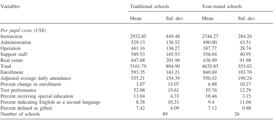
Table 2
Means and standard deviations for elementary schools’ academic year 1994–95
Variables Traditional schools Year-round schools
Mean Std. dev. Mean Std. dev.
Per pupil costs (US$)
Instruction 2932.85 449.48 2746.27 284.26
Administration 529.13 136.52 490.00 43.51
Operation 461.16 136.27 387.77 28.74
Support staff 589.53 165.53 556.04 40.95
Real estate 647.68 201.98 436.99 91.98
Total 5161.79 894.90 4635.83 353.02
Enrollment 593.35 163.21 840.69 183.70
Adjusted average daily attendance 555.21 154.39 550.42 190.24
Percent change in enrollment 1.07 15.07 6.88 10.27
Test performance 52.08 15.61 55.76 12.29
Percent receiving special education 13.04 4.33 10.46 3.15
Percent indicating English as a second language 8.38 10.21 9.4 11.04
Percent defined as gifted 7.42 4.09 7.12 0.98
Number of schools 89 26
Source: Clark County School District, District-wide school accountability report, for the school year 1994–95. See the text for a
detailed definition of the variables.
Data for this study were obtained for 115 elementary schools in the Clark County, Nevada School District for the academic year 1994–95.7All schools are within the
same district so that there is no need to adjust the model for differences in tax rates, revenues, instructional pay scales, or differences in financial administration. Of the 115 elementary schools, 89 had a traditional schedule and 26 had a year-round schedule in 1994–95. Table 2 shows the descriptive statistics for the variables included in the model, for both the traditional and year-round schedule schools. Note that the average cost per student is US$526 (about 10 percent) lower for the year-round schools than for the traditional-schedule schools. Also, the savings extend to each category of costs.
As is shown in Table 2 the average enrollment is about 42 percent higher for the year-round schools. Note that the adjusted average daily attendance for each school is nearly equal (as it should be). The change in enrollment is also substantial for year-round schools. In addition, a higher percentage (3.7) of fourth graders from year-round schools than those from traditional schools scored above the national average on the standardized tests. The year-round schedule schools also appear to have a lower percentage of students with special education needs.
7 As of the 1994–95 school year there were 123 elementary schools within the Clark County School District. Eight schools were eliminated due to incomplete data.
4. Empirical results
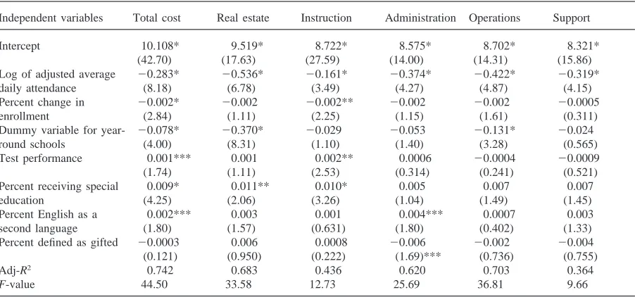
Table 3 contains heteroskedasticity-corrected Ordinary Least Squares (OLS) estimates of per pupil costs for instruction, administration, operations, support staff, real estate capital, and total per pupil cost.8
Note that the coefficient estimates are generally robust across equations and are consistent with other studies such as that of Barrow (1991) and Duncombe et al. (1995). The adjusted R-squares reveal that, depending upon the equation, 36–74 percent of the variation of average costs across schools are explained by the model. The signs and the magnitudes of the intercepts are as expected and are highly significant. Economies of size are well documented by the negative and highly signifi-cant coefficients (elasticities) on the average daily attend-ance variable. The coefficient of the test performattend-ance variable is statistically significant for the total per pupil cost and per pupil instruction cost. Alternative measures of test performance (such as mathematics, language, and reading scores entered separately) were tested with no significant alteration in the equations. As expected, higher special education requirements increase total per
Table 3
Estimates of average cost for elementary schools’ academic year 1994–95. Dependent variable: log of per pupil (average cost)a Independent variables Total cost Real estate Instruction Administration Operations Support
Intercept 10.108* 9.519* 8.722* 8.575* 8.702* 8.321*
(42.70) (17.63) (27.59) (14.00) (14.31) (15.86)
Log of adjusted average 20.283* 20.536* 20.161* 20.374* 20.422* 20.319*
daily attendance (8.18) (6.78) (3.49) (4.27) (4.87) (4.15)
Percent change in 20.002* 20.002 20.002** 20.002 20.002 20.0005
enrollment (2.84) (1.11) (2.25) (1.15) (1.61) (0.311)
Dummy variable for year- 20.078* 20.370* 20.029 20.053 20.131* 20.024
round schools (4.00) (8.31) (1.10) (1.40) (3.28) (0.565)
Test performance 0.001*** 0.001 0.002** 0.0006 20.0004 20.0009
(1.74) (1.11) (2.53) (0.314) (0.241) (0.521)
Percent receiving special 0.009* 0.011** 0.010* 0.005 0.007 0.007
education (4.25) (2.06) (3.26) (1.04) (1.49) (1.45)
Percent English as a 0.002*** 0.003 0.001 0.004*** 0.0007 0.003
second language (1.80) (1.57) (0.631) (1.80) (0.402) (1.33)
Percent defined as gifted 20.0003 0.006 0.0008 20.006 20.002 20.004
(0.121) (0.950) (0.222) (1.69)*** (0.736) (0.755)
Adj-R2 0.742 0.683 0.436 0.620 0.703 0.364
F-value 44.50 33.58 12.73 25.69 36.81 9.66
a Note: *, **, ***: significant at 0.01, 0.05, 0.10 levels, respectively. Absolute t-values are reported in parentheses. See the text for a detailed definition of the variables.
costs and its components with the exception of adminis-tration and support. Costs are also higher where there are more students with English as a second language due to an administrative cost component. More gifted stu-dents appear not to have much impact on costs.
The results also demonstrate that a change to a year-round schedule produces added cost savings. Total costs are reduced by 7.5 percent (about US$400 per pupil) after controlling for average daily attendance and test performance.9The largest impact of year-round
school-ing is on the cost of real estate capital, where there is a reduction of 31 percent in the per pupil cost. In dollar terms the cost savings is approximately US$200 per pupil. Because operating costs have large fixed cost components it is not surprising to see that there is a 12.3 percent reduction in per pupil costs of operations.
The empirical literature on school district consoli-dation reveals significant cost savings due to scale econ-omies.10As is shown in Table 3, and similar to
consoli-dation, a year-round schedule results in significant cost savings even after controlling for test performance and average daily attendance.
9 The interpretation of a dummy variable where the depen-dent variable is in logarithms can be found by subtracting one from the antilogarithm of the coefficient on the dummy vari-able: e20.07821=0.9249621=20.075.
10 Economies of scale is multidimensional and refers to quan-tity and quality aspects (student achievement, school activities, and mix of curriculum) and economies of size (see Fox, 1981; Duncombe et al., 1995).
The year-round versus traditional schedule selection process, described in Section 2, does not suggest that either endogeneity or sample selectivity is likely to be a problem. The assignment of a school to year-round by officials depends mainly on overcrowded enrollment and expected future population growth. To be certain, how-ever, let us assume that, for example, parents of a parti-cular school are very concerned about their child’s edu-cation, are active participants in the school, support year-round schooling, and help their children at home with their education. The net effect of this parental involve-ment might be a lower cost of producing a given level of student achievement. If this were the case, then it is not clear that the lower costs in these schools can be attributed solely to year-round schooling. This implies potential endogeneity of test performance and/or year-round dummy variables.11
To investigate the endogeneity/sample selection prob-lem, we performed several versions of the Hausman test (Pindyck & Rubinfeld, 1991, pp. 303–305; Maddala, 1992, pp. 506–513, 510–511). We tested for the exogen-eity of the year-round and the test performance (achievement) variables separately. We also conducted a joint test, using F-distributions, for exogeneity of the year-round and the test performance variables. The
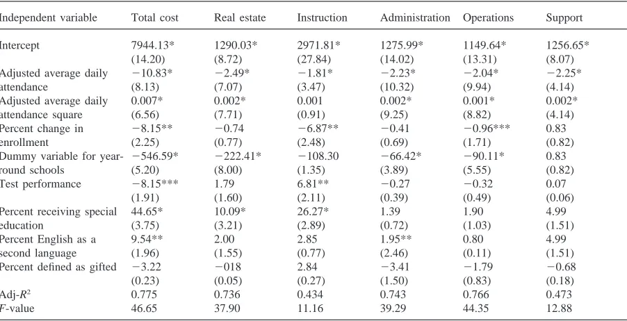
Table 4
Estimates of quadratic average cost function for elementary schools’ academic year 1994–95. Dependent variable: per pupil (average cost)a
Independent variable Total cost Real estate Instruction Administration Operations Support
Intercept 7944.13* 1290.03* 2971.81* 1275.99* 1149.64* 1256.65*
(14.20) (8.72) (27.84) (14.02) (13.31) (8.07)
Adjusted average daily 210.83* 22.49* 21.81* 22.23* 22.04* 22.25*
attendance (8.13) (7.07) (3.47) (10.32) (9.94) (4.14)
Adjusted average daily 0.007* 0.002* 0.001 0.002* 0.001* 0.002*
attendance square (6.56) (7.71) (0.91) (9.25) (8.82) (4.14)
Percent change in 28.15** 20.74 26.87** 20.41 20.96*** 0.83
enrollment (2.25) (0.77) (2.48) (0.69) (1.71) (0.82)
Dummy variable for year- 2546.59* 2222.41* 2108.30 266.42* 290.11* 0.83
round schools (5.20) (8.00) (1.35) (3.89) (5.55) (0.82)
Test performance 28.15*** 1.79 6.81** 20.27 20.32 0.07
(1.91) (1.60) (2.11) (0.39) (0.49) (0.06)
Percent receiving special 44.65* 10.09* 26.27* 1.39 1.90 4.99
education (3.75) (3.21) (2.89) (0.72) (1.03) (1.51)
Percent English as a 9.54** 2.00 2.85 1.95** 0.80 4.99
second language (1.96) (1.55) (0.77) (2.46) (0.11) (1.51)
Percent defined as gifted 23.22 2018 2.84 23.41 21.79 20.68
(0.23) (0.05) (0.27) (1.50) (0.83) (0.18)
Adj-R2 0.775 0.736 0.434 0.743 0.766 0.473
F-value 46.65 37.90 11.16 39.29 44.35 12.88
a Note: *, **, ***: significant at 0.01, 0.05, 0.10 levels, respectively. Absolute t-values are reported in parentheses.
centage of students receiving free meals and the percent-age of teachers with a master’s degree were used as instrumental variables.12 The null hypothesis that the
year-round and the test performance variables are not exogenous, or that there is no simultaneity, could not be rejected for any of the six equations. In addition, the significance level and the magnitude of the test perform-ance and the year-round variables did not change. Thus, we conclude that there is not a serious endogeneity/sample selection problem regarding year-round and test performance variables in our data set.
5. Conclusion
As expected, the more intensive use of a school facility through the implementation of a year-round schedule results in significant cost savings. The savings are largest in the fixed cost area of real estate and oper-ations. We focus in this paper on the real estate costs
12 The sample revealed a high correlation between test per-formance and percentage receiving free meals variables. Thus, while not correlated with parental decisions about location, the percentage receiving free meals is an excellent “instrument” for the test performance variable. The sample also revealed that the percentage of teachers with a master’s degree is correlated with the year-round status. This variable is used as the instrument for the year-round variable.
and find that there are potential savings of about US$200 per student per year that result from a change to a year-round schedule from a traditional schedule. Since there are 52,800 students remaining in traditional schedule facilities in the County, the potential cost of real estate savings is US$10,500,000. Although it may be imprac-tical or even logisimprac-tically impossible to convert every school to a year-round schedule, the estimate of savings from this study can be used to calculate the potential savings from converting any single existing or proposed facility to this schedule.
Appendix A
Table 4
References
Barrow, M. M. (1991). Measuring local education authority per-formance: a frontier approach. Economics of Education
Review, 10, 19–27.
Callan, S. J., & Santerre, R. E. (1990). The production charac-teristics of local public education: a multiple product and input analysis. Southern Economic Journal, 57, 468–480. Deller, S. C., & Rudnicki, E. (1993). Production efficiency in
elementary education: the case of Maine public schools.
Economics of Education Review, 12, 45–57.
savings from school district consolidation: a case study of New York. Economics of Education Review, 14, 265–283. Fox, W. F. (1981). Reviewing economies of size in education.
Journal of Education Finance, 6, 273–296.
Geisert, G. (1990). Teacher union involvement in year-round schooling. Government Union Review, 11, 30–41. Hanushek, E. A. (1986). The economics of schooling:
pro-duction and efficiency in public schools. Journal of
Econ-omic Literature, 24, 1141–1177.
Jimenez, E. (1986). The structure of education costs: multipro-duct cost functions for primary and secondary schools in Latin America. Economics of Education Review, 5, 25–39. Kenny, L. (1982). Economies of scale in schooling. Economic
Education Review, 2, 1–24.
Kumar, R. (1983). Economies of scale in school operation: evi-dence from Canada. Applied Economics, 15, 323–340. Levin, H. M. (1974). Measuring efficiency in educational
pro-duction. Public Finance Quarterly, 2, 3–24.
Maddala, G. S. (1992). Introduction to econometrics. (2nd ed.). New York: Macmillan.
Pindyck, R. S., & Rubinfeld, D. L. (1991). Econometric models
and economic forecasts. (3rd ed.). New York: McGraw-Hill.
Watt, P. A. (1980). Economies of scale in schools: some evi-dence from the private sector. Applied Economics, 12, 235–242.