Vol. 41 (2000) 117–146
Adaptation and convergence of behavior in repeated
experimental Cournot games
Stephen Rassenti
a, Stanley S. Reynolds
b, Vernon L. Smith
a,b,∗,
Ferenc Szidarovszky
caEconomic Science Laboratory, McClelland Hall, University of Arizona, Tucson, Arizona 85721, USA bDepartment of Economics, McClelland Hall, University of Arizona, Tucson, Arizona 85721, USA cDepartment of Systems and Industrial Engineering, University of Arizona, Tucson, Arizona 85721, USA
Received 30 March 1999; received in revised form 30 March 1999; accepted 8 April 1999
Abstract
This research examines results from laboratory experiments in which five human subjects par-ticipate as sellers in a Cournot oligopoly environment. The central issue is whether repeated play among a group of privately informed subjects will lead to convergence to a unique, static, nonco-operative Nash equilibrium. The experiments were designed so that the implications of different hypotheses about adaptation and convergence, such as the best response dynamic and fictitious play, could be distinguished. The results provide, at best, only partial support for the hypothesis that behavior of privately informed subjects will converge to the static Nash equilibrium when play is repeated. Total output averaged over time periods and across experiments is greater than, but still close to, predicted equilibrium total output. However, observed intertemporal variation in total output and heterogeneity in individual choices are inconsistent with convergence to the static Nash equilibrium. ©2000 Elsevier Science B.V. All rights reserved.
JEL classification:Experimental economics 026; Game theory 215; Industrial organization 610 Keywords:Cournot games; Oligopoly; Nash equilibrium; Learning
1. Introduction
The concept of equilibrium is central to most theories of economic behavior. Many of these theories are based on game-theoretic models that take the strategic incentives of par-ticipants into account when formulating predictions of behavior. One concern about the
∗Corresponding author..
application of equilibrium theories of behavior involves convergence of actual behavior to predicted equilibrium behavior. Suppose that a group of decision-makers are in an environ-ment in which they do not initially possess all of the information required to arrive at the deci-sions predicted by the equilibrium.1 Would their behavior eventually converge to predicted equilibrium behavior through some process of learning and adaptation of decision-making based upon observations of the environment, or would the adaptation process lead away from equilibrium toward some other outcome?
This paper reports on a series of laboratory experiments that were designed to shed some light on the issue of convergence to equilibrium behavior. The environment we utilize is an operationalized version of the Cournot oligopoly model of output choice. The Cournot model is a good candidate for experimental testing because it is one of the simplest of a large number of market models whose predictions rest crucially on the notion of equilibrium. Many analyses of the effects of horizontal mergers are based upon the Cournot framework (see Farrell and Shapiro, 1990 and the references therein), and much of applied industrial organization uses the Cournot model as a benchmark. Our experimental results provide further insight into the nature of strategic interaction among firms in oligopoly markets.
In addition to its relative simplicity, the Cournot model possesses an interesting set of equilibrium and convergence predictions. Our experiments utilize five seller subjects who repeatedly play a Cournot game of output choice. There is a unique (pure strategy) Nash equilibrium for the corresponding static game of output choice. With repeated play, be-havior may or may not converge to this Nash equilibrium, depending upon the learning or adjustment process utilized by subjects. For example, if subjects utilize the best response dy-namic (the adjustment mechanism proposed by Cournot) then behavior would not converge to the static Nash equilibrium. Some alternative adjustment processes, such as fictitious play, do yield convergence to the static Nash equilibrium. Our experimental design offers the opportunity to distinguish between competing theories of learning or adjustment.
A few prior output-choice experiments have particular relevance for our study.2Fouraker and Siegel (1963) report on triopoly quantity setting experiments under incomplete infor-mation. Payoffs are based on a simple homogeneous product model with linear demand and zero marginal cost. Information is incomplete because each subject is uninformed about rivals’ payoffs. In each experiment, a fixed group of three subjects make choices over a sequence of periods. The single period Nash equilibrium (i.e., Cournot, 1960) prediction performs well as a predictor of total output in these triopoly experiments, although total output tends to be somewhat higher than the Nash equilibrium (NE) prediction.3 There is less support for the NE prediction of equal individual output choices, with substantial
1Some economic models of behavior recognize this lack of information explicitly and include the way in which agents utilize and react to new information as part of the equilibrium. For instance, this information updating process is an explicit part of the decision-making process for a sequential equilibrium or a Bayes Nash equilibrium.
2There are many other quantity setting oligopoly experiments that we could cite. However, most of these are duopoly experiments which introduce a high potential for cooperative behavior, and, in many instances, focus on attempts to implement cooperation. See, for example, Selten et al. (1997). We attempt to limit the potential for cooperative behavior by running experiments with five seller subjects.
variation in output choices across subjects within experiments and over time for individual subjects. Wellford (1990) reports on 10 oligopoly quantity setting experiments with five seller subjects. The setup was similar to the incomplete information design in Fouraker and Siegel. However, subjects have (identical) increasing marginal costs in Wellford, in con-trast to the constant marginal costs in Fouraker and Siegel. Total output tended to fluctuate between the Cournot and competitive levels, with average total output about 15 percent greater than the Cournot prediction. Individual output choices were not reported. However, the values of the Herfindahl index reported by Wellford indicate substantial departures from the equal-outputs Cournot prediction.4
Two recent studies of Cournot experiments are mainly concerned with stability and con-vergence issues. Cox and Walker (1998) report experiments in which a group of subjects were randomly matched to form two-seller duopolies in each trading period. Subject pay-offs are defined to yield reaction functions that are stable with respect to the best response dynamic in one treatment and unstable in another treatment. There was a sharp difference between behavior in the stable and unstable duopoly experiments. After a few early peri-ods, output choices in the stable duopolies are at or near the equilibrium. In the unstable duopolies, output choices are rarely near the interior equilibrium. A paper closely related to our work is the Huck et al. (1998) study of Cournot experiments with symmetric (and con-stant) marginal costs and four seller subjects. In one treatment the best response dynamic is unstable, as it is for all of our experiments. A second treatment generates inertia in choices by requiring a subject to keep their output unchanged from its previous period level with positive probability. The best response dynamic is stable in the treatment with inertia. Huck et al., 1998, do not find important differences in behavior across these two treatments. They observe that,
Play converges roughly to the Cournot equilibrium prediction, regardless of whether the best response dynamic predicts stability or explosive fluctuations (Huck et al., 1998, p. 10).
This observation may overstate the extent of convergence, however. Based on the graphs of total output, five out of 12 experiments seem to exhibit output fluctuations for the duration of the experiment. Also, the Cournot (Nash) equilibrium predicts equal individual outputs for the four sellers. Huck et al., 1998 do not report statistics on individual output choices.
2. Experimental environment
We have operationalized a version of the Cournot oligopoly model of output choice for the experiments. Five subjects participate in each experiment, with each subject taking on the role of a seller. At the beginning of each trading period, each subject chooses a quantity of output to sell. These choices are made simultaneously. A market price is determined by
an inverse demand function. A subject’s payoff for a trading period is equal to the output chosen by the subject times the difference between the market price and the (constant) marginal cost for the subject. A new trading period begins after the subjects have observed the market outcome.
The experiments were run on a local area network program called OLIGOP. A copy of the instructions for these experiments appears in the Appendix A. The experimental environment was constructed with several features that permit us to focus on how subjects learn about the environment over time and adapt their decisions in response to what they observe.
2.1. Repeated trials
Each experiment has repeated trials (or trading periods) with a fixed group of subjects who interact with each other in each period. We investigate the extent to which the behavior of a fixed group of subjects who interact with each other repeatedly will converge to a static noncooperative Nash equilibrium (NE) prediction. This is in contrast to Cox and Walker (1998) who re-match subjects to form new pairs in each trading period. An environment of repeated play with a fixed group of subjects has been used in prior experimental studies of convergence to equilibrium, such as Van Huyck et al. (1990, 1994). However, these studies focused on the role of the adaptation and adjustment process for selection of equilibrium when there are multiple (static) equilibria. Our interest is in convergence to equilibrium when there is a unique static equilibrium.
The (baseline) payoff conditions remain constant during the repeated trials within an experiment. This fixed payoff condition permits us to focus on how subjects are adapting their decisions over time based on how they improve their understanding of the (fixed) payoff conditions and on what they learn about how other subjects in the market are behaving.
Each experiment was run for a total of 75 periods.5 This is a large number of trading
periods, compared with many other laboratory experiments. The long time horizon allows plenty of time for the market to converge, if convergence is ultimately to occur. A long time horizon also allows for the possibility of estimation of a time series model of the data generating process. Subjects are not informed about the termination rule for the experiment.
2.2. Payoff information
The demand function is public information for subjects. Each subject is informed (and is informed that other subjects are also informed) that the market price of output is a particular function of the sum of outputs selected by the subjects. Cost information is private for each subject. Each subject is informed about their (constant) marginal cost of output. However, no information is provided about the marginal costs of other subjects (not even information about the distribution of costs). The instructions inform subjects that they should not necessarily assume that other subjects have costs equal to their own costs. In fact,
subjects are assigned different marginal costs within each experiment.6 As a consequence,
payoffs are asymmetric and there are no symmetric Nash equilibria. Subjects would not be able to (accurately) infer that their rivals have payoffs equal to their own and adopt a symmetric Nash equilibrium strategy, as is possible in some experimental setups.
This private payoff condition has two important implications for behavior. First, it is not possible for subjects to compute (or estimate) noncooperative Nash equilibrium outputs and play the corresponding equilibrium strategies. If choices are to converge to a Nash equilibrium then this convergence must occur based on how subjects adapt their decisions over time in response to observed history rather than as a result of a priori reasoning about what the ‘correct’ (i.e., equilibrium) choices must be. Second, it is not possible for subjects to compute a joint profit maximizing selection of outputs. It is possible that observed play would converge to something like a joint profit maximizing solution, since there are repeated trials with a fixed group of subjects. However, this would require that subjects understand (at least approximately) what the joint profit maximizing solution is and that subjects learn how to interpret their rivals’ actions. For example, does a low output choice by a rival indicate a cooperative gesture by the rival or does it indicate that the rival has a relatively high marginal cost, so that the rival has a selfish incentive to keep its output low?
2.3. Market information
At the end of a trading period subjects observe the market price of output, the output of their rivals, and their own payoff. The computer screen lists up to eight periods of market outcomes. The amount of information provided about rivals’ choices is a treatment condi-tion. We ran some experiments in which subjects observe the choices of each one of their rivals. These are designated as SHOW experiments. We ran another group of experiments in which subjects observed only the total output chosen by their rivals. These are called NO-SHOW experiments.
Rivals’ choices enter into a seller’s payoff function only through the total output chosen by the rivals; the way in which output is divided among rival sellers does not affect a seller’s payoff. For this reason, most of the learning and decision adjustment processes that have been proposed for the Cournot oligopoly environment depend only on aggregate output of rivals in previous periods. However, the provision of information about the individual choices of rivals may influence the learning process. One example of this is the strategy of imitating relatively successful strategies of rivals. Vega-Redondo (1997) shows that an evolutionary process in which firms can imitate in this way yields convergence to the competitive equilibrium.7This suggests the hypothesis that our SHOW experiments would
yield higher outputs (lower output prices) than NO-SHOW experiments.
A quite different hypothesis emerges from the oligopoly literature on collusion. Stigler (1964) argues that greater access to information about outputs of individual firms would
6Subjects have constant, equal marginal cost in Huck et al. (1998). While their instructions do not explicitly state that all subjects have the same costs, their instructions may be interpreted as implying that other subjects have identical costs.
facilitate (either tacit or explicit) collusion, because this information would increase the chances that defection from collusion would be detected. This view of information and collusion suggests the hypothesis that our SHOW experiments would yield lower outputs than NO-SHOW experiments, because the SHOW condition would facilitate tacit collusion.
2.4. Number of subjects
We chose to have a relatively small number of subjects in this environment so that subjects would recognize the fact that payoffs were interdependent. We did not want an environment in which a subject would view their own choice as being an insignificant part of an overall market process. On the other hand, since one of our primary objectives is to examine hypotheses concerning convergence to a static, noncooperative Nash equilibrium, we wanted to have more than two or three seller subjects. A very small group of subjects would be more likely to implement some type of cooperative outcome when there are repeated trials, even in this incomplete information environment, than would a larger group of subjects. Also, a number of seller subjects greater than three permits us to distinguish between the predictions of two of the adjustment hypotheses (see below).
2.5. Working capital and bankruptcy
It is possible for a subject to receive a negative payoff in a trading period, since the market price may fall below a seller subject’s marginal cost.8 Therefore, we provided subjects with
starting working capital equal to approximately two periods worth of Nash equilibrium earnings. Also, we allowed a subject’s accumulated earnings to become negative. A subject was declared bankrupt if their accumulated earnings remained negative for more than five periods. In case of bankruptcy, the experiment would continue with the remaining solvent subjects. There were no cases of bankruptcy for the working capital provision level and bankruptcy rule that we used in the experiments that are reported in this paper.
3. Model parameters, equilibrium and convergence
Each subject chooses a level of output in each trading period. The market price is deter-mined by a linear inverse demand function. The market price in periodtis,
p(xt)=max (
0, a−b 5 X
i=1 xit
)
(1)
wherexitis (nonnegative) output chosen by subjectiin periodt,xt is the vector of outputs int, andaandbare demand parameters. Subjectihas constant marginal cost of outputci and no fixed costs. The profit payoff in experimental pesos for subjectiin periodtis,
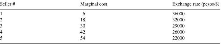
Table 1 Parametersa
Seller # Marginal cost Exchange rate (pesos/$)
1 6 36000
2 18 32000
3 30 29000
4 42 26000
5 54 22000
aInverse demand:p=540−X;X=Total output.
Table 2
Nash equilibrium benchmarka
Seller # Output Payoff (pesos) Payoff ($)
1 109 11881 0.330
2 97 9409 0.294
3 85 7225 0.249
4 73 5329 0.205
5 61 3721 0.169
Total output 425
Market price 115
aAll figures are for a single trading period.
p(xit, x−i,t)=[p(xt)−ci]xit (2)
wherex−i,tis the vector of outputs chosen by rival subjects int.
The values for the demand and cost parameters that were used in the experiments are listed in Table 1. These parameters yield a unique noncooperative Nash equilibrium for the one-shot, complete information constituent game. This is in contrast to the unstable case in Cox and Walker (1998). Their unstable interior equilibrium co-exists with two stable corner equilibria in which one firm has zero output. The failure of choices to converge to the unstable interior equilibrium in the Cox and Walker experiments could be attributed to subjects’ inability to coordinate their actions to select one of the three equilibria.
The outputs and payoffs for the NE are listed in Table 2. Note that levels of output in equilibrium are ranked in inverse order of levels of marginal costs.9 Also, each seller has
positive output in equilibrium. There are no ‘corner’ equilibria (i.e., equilibria with zero output for one or more sellers) for these parameters.
In the absence of information about rivals’ costs, subjects could not be expected to choose NE outputs initially. In fact, even with knowledge of rivals’ payoffs, a wide range of output choices may be reasonable at the beginning of a sequence of plays. For example, Bernheim (1984) proposes that game players would adopt rationalizable strategic behavior. Roughly speaking, rationalizable strategies are best responses based on reasonable subjective
sessments of what rival players might do. For a Cournot duopoly, the set of rationalizable strategies corresponds to the unique NE.
However, for our 5 player Cournot oligopoly, a player’s set of rationalizable strategies is any output level between zero and the player’s monopoly output (see Bernheim, 1984, pp. 1024–1025). This suggests that a subject may view a wide range of outputs as ‘reasonable’ initial choices in this environment.
As subjects gain experience making decisions and observe what rival subjects do, they may learn more about the environment and adjust their behavior over time. A variety of decision adjustment and adaptation processes have been proposed in the literature on learn-ing and convergence in games. We discuss several of these processes in the context of our Cournot experimental environment below.
3.1. Best response dynamic
This adjustment process has been analyzed for many models and was in fact the ad-justment process originally suggested by Cournot (Cournot, 1960) in his duopoly analysis. Under the best response dynamic each subject sets his current output equal to the best (i.e., current period payoff maximizing) response to the last period outputs of his rivals. Cournot demonstrated that this adjustment process was stable and converged to the unique NE for a duopoly with linear demand and constant marginal cost.
For our simple linear demand and cost model with five sellers, the best response dynamic yields the following adjustment process:
This adjustment process may be written in vector form as,
xt =h+H xt−1 (4)
wherehis a 5×1 vector of parameters andHis a 5×5 matrix with zeros on the diagonal and each off-diagonal term equal to−1/2.10 Hhas eigenvalues−2 and 1/2 repeated four times. This is an unstable difference equation, sinceHhas an eigenvalue that exceeds 1 in absolute value. This means that the best response dynamic does not yield convergence to the NE for our experimental environment. If subjects selected their best response to last period rival outputs then they would collectively ‘overshoot’ the NE and eventually begin to oscillate between zero output and a high output with a zero price. This result is an illustration of the general instability result found by Theocharis (1960) and Fisher (1961).
3.2. Partial adjustment to best responses
If subjects lack confidence in their forecasts of rivals’ behavior or if decision-making involves some element of inertia then subjects may use an adjustment process that is more
conservative than the best response dynamic. One such process is partial adjustment to a subject’s best response in each period. A simple linear specification would be a weighted average of a subject’s last period output and the subject’s best response to rivals’ last period output:
xit =dixi,t−1+(1−di)Ri(x−i,t−1) (5)
This process yields a first-order linear difference equation of the form of (4) where rowiof the matrix of coefficients now has a diagonal element equal todiand off-diagonal elements equal to (di−1)/2. This difference equation is asymptotically stable and converges to the NE if all subjects have a common value for the adjustment parameter,di, and this parameter is between 1/3 and 1. Szidarovszky et al. (1994) derive a general stability condition for heterogeneous adjustment rates. If some subjects place a large weight on their best response (smalldi) then this condition requires that other subjects place a sufficiently small weight on their best response (largedi) in order to stabilize the system. Thus, this modified form of the best response dynamic yields convergence to the NE as long as all subjects do not adjust to their best response too quickly.
There is some experimental evidence to suggest that partial adjustment to best responses to last period rivals’ choices is more likely to be observed than complete adjustment to these best responses. Kruse et al. (1994) report on a series of four-seller posted pricing experiments in which seller subjects faced production capacity constraints. A regression of the form of Eq. (5) was run for the price adjustment of each one of the 80 subjects in the experiments. The characteristic result was that the estimateddi parameter was positive and significantly greater than 0. A typical value fordiwas 0.8 or greater.
3.3. Fictitious play
Under fictitious play (Brown, 1951) each subject would take the observed frequency distribution of past choices of rivals into account when choosing their current output. Each subject is assumed to choose current output to maximize their expected payoff, where rivals’ choices are assumed to be drawn from the empirical frequency distribution of their past choices. The expected profit of output choicexi for subjectiin periodtwould be,
t−1 X
s=1
p(xi, x−i,s)
t−1 (6)
Note that 1/(t−1) represents the frequency probability of one choice out oft−1 total choices. The analysis of stability of fictitious play is simplified by definingyj ,t−1as the average
of subjectj’s output choices in periods one through t−1. The expected payoff for i in expression (6) may now be rewritten as,
t−1
We have already shown that the best response dynamic is unstable for our 5 player envi-ronment. However, Thorlund-Petersen (1990) shows that fictitious play generates a stable output path that converges to the static Nash equilibrium for our oligopoly environment. Having players make a best response to a forecast based on historical averages of rivals’ choices mitigates the ‘overshooting’ problem that occurs with the best response dynamic.
3.4. Adaptive learning
Milgrom and Roberts (1991) adaptive learning formulation represents a general class of decision adjustment processes. A player’s sequence of choices is consistent with adaptive learning if the player eventually chooses only strategies that can be justified in terms of its rivals’ past play. This justification is based on choosing strategies that are in an un-dominated set of strategies when rivals’ strategies are restricted to a subset of historically observed strategies. The best response dynamic and fictitious play are two examples of adaptive learning processes.11 Milgrom and Roberts show that if sequences of choices sat-isfy adaptive learning for all players and the sequence converges then the convergent point must be a Nash equilibrium. However, not all choice behavior that satisfies the definition of adaptive learning will converge (consider for example, the non-convergence of the best response dynamic). Milgrom and Roberts’ definition of adaptive learning cannot be used in a direct manner to categorize observed play in an experimental setting. An infinite sequence of observations would be required to apply their definition directly.
Sophisticated learning is another class of learning processes characterized by Milgrom and Roberts (1991). As with adaptive learning, the idea is that a player’s strategy choices would eventually be in a set of undominated strategies, given some restriction on the set of rivals’ strategies. However, the set of rivals’ strategies includes strategies that are undom-inated for them, as well as rivals’ historically observed strategies. This can be viewed as a more sophisticated mode of play than adaptive learning since it permits a player to anticipate how its rivals might react to past play, rather than presuming that rivals will behave as they did in the past.12
4. Results and analysis
We report on three types of experiments. The ‘75-SHOW’ experiments were run for 75 periods and subjects were able to observe the past output choices of each one of their rivals. The ‘75-NO SHOW’ experiments were run for 75 periods and subjects could observe only
11Adaptive learning does not require that agents make payoff-maximizing choices, given their forecasts. It merely requires that agents converge to choices that are close to optimizing choices, given the play that they have observed. A non-optimizing adaptation process, such as partial adjustment to best responses could potentially be classified as adaptive learning.
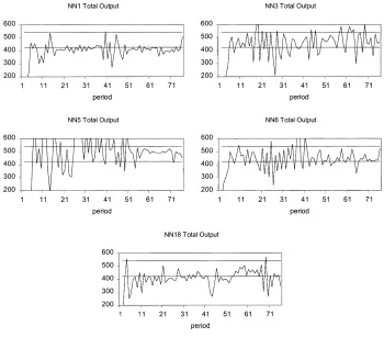
Fig. 1. Time series plots for total output.
the past total output of rivals. The ‘15/60-SHOW’ experiments were run for 15 periods with a set of parameters different from the parameters in Table 1, followed by 60 periods with the parameters from Table 1. Subjects were able to observe the past choices of individual rivals in this type of experiment. We have run five experiments for each of the three types of experiments. The raw data are available from the authors upon request.
4.1. Aggregate output
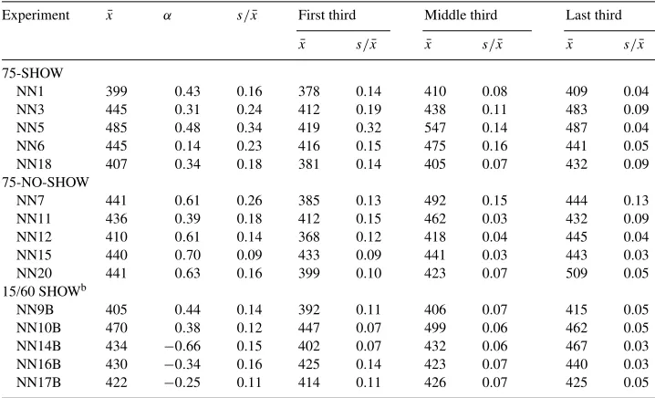
Time series plots for total output are provided in Figs. 1–3. The lower solid line is the NE prediction; the upper solid line is the total output level that yields a zero price. Summary statistics for total output are provided in Table 3.
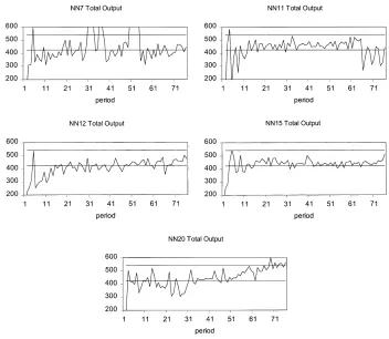
Fig. 2. Time series plots for total output.
Total outputs, taken as an average across experiments for each type of experiment, are slightly higher than the Nash equilibrium prediction of 425 units. The average for 75-SHOW experiments is 2.5 percent higher than the NE benchmark, the average for the 75-NO SHOW is 2 percent higher than the NE benchmark, and the average for the 15/60-SHOW is 1.7 percent higher than the NE benchmark. In addition, average total output during the last one-third of each experiment tends to be greater than average total output for the entire experiment. So, there is a central tendency for total output to be somewhat above the NE benchmark (so that average price tends to be below the NE price).
Sample autocorrelation statistics (α) are also reported in Table 3. This statistic is positive for 12 out of 15 experiments. This is noteworthy because both the best response dynamic and fictitious play would generate negative serial correlation (although with fictitious play the correlation between successive periods would approach zero as time passes). So, the actual movement of total output over time appears to be inconsistent with both the best response dynamic and fictitious play, for most experiments.
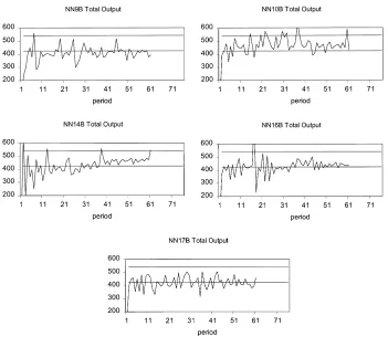
Fig. 3. Time series plots for total output.
experiment in which total output was substantially less than NE total output for more than a few periods.
The treatment conditions involving provision of information about rivals’ outputs and prior experience did not have a significant effect on total output levels. Thus, there is no evidence to support the imitation hypothesis, which states that SHOW experiments would yield higher outputs. Likewise, there is no evidence to support the collusion and information hypothesis, which states that SHOW experiments would yield lower outputs due to tacit collusion. Experiments in which the subjects had 15 periods of experience with a different Cournot environment (15/60 SHOW) exhibited less variability in total output over time than experiments in the other treatments.
4.2. Individual behavior
Table 3
Summary statistics for total outputa
Experiment x¯ α s/x¯ First third Middle third Last third ¯
ax¯: Mean output;α: Sample autocorrelation;s: Sample standard deviation. bLast 60 periods.
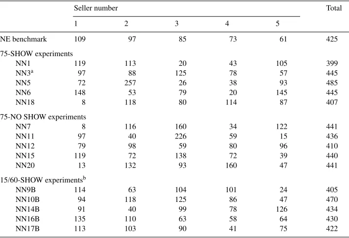
had the greatest average output. Moreover, the observed patterns in the distributions of outputs across subject sellers persist throughout most experiments. This means that observed behavior for individual subject sellers is not converging to the static Nash equilibrium predictions for individual output choices in these experiments.
Individual behavior is explored in more detail by estimating the decision rules used by subjects. Decision rules are assumed to take the form,
xit =β0i+β1it+β2ixi,t−1+β3izi,t−1+β4izi,t−2+eit (8) wherezitis the sum of outputs intfori’s rivals andeitis a residual term. This form permits a subject’s output choice to depend on lagged own and rivals’ output and twice lagged rivals’ output. Longer lag lengths yielded insignificant coefficients in the estimation for almost all subjects. Thetterm allows for a time trend. The residual term, eit, captures error in estimating the true decision rule as well as random experimentation by subjects.
The individual output series is nonstationary for many subjects.13 Therefore, we took
first differences to transform the decision rule in (8) into,
1xit =β1i+β2i1xi,t−1+β3i1zi,t−1+β4i1zi,t−2+εit (9) where1is the first-difference operator. Eq. (9) was estimated using the Seemingly Unrelated Regressions method for each group of five subjects in an experiment. This allows for within-period correlation of the residual terms for the five subjects within an experiment.
Table 4 Average outputs
Seller number Total
1 2 3 4 5
NE benchmark 109 97 85 73 61 425
75-SHOW experiments
aExchange rates were assigned differently: Seller 1 (36,000 pesos/$); Seller 2 (29,000 pesos/$); Seller 3 (22,000 pesos/$); Seller 4 (26,000 pesos/$); Seller 5 (32,000 pesos/$).
bLast 60 periods.
Table 5
Decision rule estimationa,b
Formc 1x
it=β1i+β2i1xi,t−1+β3i1zi,t−1+β4i1zi,t−2+εit
Individual results Number of subjects whose behavior permits rejection of the (75 subjects) Null hypothesis (out of 75)
5% level 1% level
H0:β3i= −1/2 72 71
H0:β3i=0d 14 12
H0:β3i=β4i=0 50 48
H0:β2i=0e 11 8
aPooled estimation results (standard errors in parentheses): 1xit=0.537 −0.4171xi,t−1−0.0301zi,t−1−0.0241zi,t−2
(0.514) (0.013) (0.007) (0.006) . bN: 5025 Observations; AdjustedR2: 0.182; D.W. statistic: 2.164.
cx
itis periodtoutput for selleri;zitis the sum of outputs fori’s rivals int. dOne-tailed test, with alternative hypothesis,β
3i<0. eOne-tailed test, with alternative hypothesis,β
2i> 0.
for a subject. However, more subjects had negative, significant coefficients on own lagged output.
Estimation results for a pooled sample consisting of all subjects are also reported in Table 5. This can be thought of as estimating a common decision rule for all subjects, based on all of the experimental data. On average, there is a small, negative response to lagged changes in rivals’ output. There is a negative response to lagged changes in own output and a positive time trend. The pooled estimation results mask a large amount of heterogeneity in individual decision rules. Coefficient estimates varied widely across subjects for all four coefficients.
The decision rule estimation results reveal some important characteristics of subjects’ decision making. However, they do not reveal the source of the failure of individual outputs to converge to NE outputs. Heterogeneity in adjusting could contribute to nonconvergence, but it would not necessarily have that effect (recall partial adjustment results). The apparent failure of about one-third of subjects to respond to changes in rivals’ output may be im-portant. Some subjects who do respond to lagged changes in rivals’ output make a positive response. Any convergent adjustment process would require subjects to take their rivals’ actions into account when choosing their own output. However, it may be that we fail to detect a response to rivals’ output changes in some cases because the decision rule we es-timate is misspecified. Some subjects may use a nonlinear decision rule and/or a different lag structure for rivals’ output.
5. Summary and conclusions
Total output averaged over time periods and across experiments is greater than, but still close to, predicted Nash equilibrium (NE) total output. This is consistent with results from other Cournot experiments (with more than two sellers) reported in Fouraker and Siegel (1963); Wellford (1990) and Huck et al. (1998). There was substantial intertemporal varia-tion in total output within experiments that diminished slightly as experiments progressed. There seems to have been less intertemporal variation in output in the (no inertia) experi-ments reported in Huck et al. (1998). This may have been due to their symmetric cost design, in contrast to our use of asymmetric cost assignments.14 Neither the best response dynamic nor partial adjustment to best responses are capable of explaining the output fluctuations observed in our experiments. For example, there was typically positive correlation of output over time, whereas best responses and partial adjustment to best responses predict negative correlation. Nothing like successful collusion was observed.
The most significant failure of convergence to NE is for individual output choices. While total output is typically near the NE level, individual outputs are often far from predicted NE levels, even after many periods. This is consistent with prior experimental results for sym-metric Cournot oligopolies in Fouraker and Siegel (1963) and Wellford (1990). Estimation of individual decision rules reveals a great deal of heterogeneity in subjects’ decision-making. In some respects, out results are reminiscent of the Cox and Walker (1998) results for un-stable Cournot duopolies. They also found the unun-stable interior NE to be a poor predictor of individual behavior. However, their unstable design also had two corner Nash equilibria. The failure of the interior NE to predict behavior may have been due to the presence of other equilibria. Our results show that the NE predicts individual behavior poorly in an environment with asymmetric costs and a unique, but unstable Nash equilibrium.
A potentially promising way to explain our results might come from the concept of quantal response equilibrium (QRE), developed by McKelvey and Palfrey (1995). The QRE alters the conventional game-theoretic formulation to permit a player to choose actions that yield higher expected payoffs with higher probabilities, rather than choose the single action that yields the highest payoff. Such a theory can be consistent with heterogeneity in individual decisions, while not necessarily inconsistent with Nash equilibrium predictions of aggregate behavior.15 One aspect of our experimental results that may be problematic for this type
of theory is the persistence of individual choices over time. A subject who chooses a low (high) output in one period is likely to choose low (high) outputs in future periods. This kind of persistence is not predicted by the QRE.
An important theme in recent Industrial Organization research is that market outcomes are strongly influenced by firm-level heterogeneity (see, for example, Klepper and Graddy, 1990 and Berry et al., 1995). Differences across firms in productivity and product qualities induce differences in profitability, which in turn influence the number of surviving sellers and the distribution of their sizes at any point in time. In empirical studies, the factors that influence this heterogeneity are typically not observed directly, but instead are inferred from market outcomes under the maintained hypothesis of equilibrium behavior. Our experimental results
14This difference may also be related to subjects’ ability to infer that costs were symmetric in Huck et al. (1998) Cf ft. # 7.
suggest that individual variability in behavioral strategies may also contribute to asymmetric distributions of market shares. In a Cournot oligopoly, seller subjects with the same payoffs in the same kind of market environment adopted quite different behavioral strategies. The heterogeneity in behavioral strategies coupled with individual differences in marginal costs contributed to observed asymmetric market share distributions. Behavioral heterogeneity may also contribute to the evolution of observed asymmetric market share distributions in naturally occurring markets.
Acknowledgements
We thank John Van Huyck for comments on a previous draft. George Vachadze and Eric Von Dohlen provided able assistance with the data analysis. This work was supported, in part, by grant SES-9023055 from the National Science Foundation.
Appendix A. OLIGOP instructions
Hello, Welcome to the ECONOMIC SCIENCE LABORATORY
Since you will be paid for your participation in on experiment, we are required to record some personal information for administrative purposes. However, in the experiment you will be entirely anonymous since we keep track of subjects using only their seat numbers.
References
Bernheim, B.D., 1984. Rationalizable strategic behavior. Econometrica 52, 1007–1028.
Berry, S., Levinsohn, J., Pakes, A., 1995. Automobile prices in market equilibrium. Econometrica 63, 841–890. Brown, G., 1951. Iterative solutions of games by fictitious play. In: Koopmans, T. (Ed.), Activity Analysis of
Production and Allocation. Wiley, New York.
Cournot, A., 1960. Recherches sur les principes mathematiques de la theorie des richesses. Hachette, Paris, 1838. Researches into the Mathematical Principles of the Theory of Wealth (N.T. Bacon, Trans.). Kelley, New York. Cox, J., Walker, M., 1998. Learning to play Cournot duopoly strategies. Journal of Economic Behavior and
Organization 36, 141–161.
Farrell, J., Shapiro, C., 1990. Horizontal mergers: an equilibrium analysis. American Economic Review 80, 107– 126.
Fisher, F., 1961. The stability of the Cournot oligopoly solution: the effects of speeds of adjustment and increasing marginal costs. Review of Economic Studies 28, 125–135.
Fouraker, L., Siegel, S., 1963. Bargaining Behavior. McGraw-Hill, New York.
Huck, S., Norman, H., Oechssler, J., 1998. Stability of the Cournot Process — Experimental Evidence. Mimeo, Humboldt University, Berlin.
Klepper, S., Graddy, E., 1990. The evolution of new industries and the determinants of market structure. Rand Journal of Economics 21, 27–44.
Kruse, J., Rassenti, S., Reynolds, S., Smith, V.L., 1994. Bertrand-Edgeworth competition in experimental markets. Econometrica 62, 343–361.
McKelvey, R., Palfrey, T., 1995. Quantal response equilibria in normal form games. Games and Economic Behavior 7, 6–38.
Milgrom, P., Roberts, J., 1991. Adaptive and sophisticated learning in normal form games. Games and Economic Behavior 3 (1), 82–100.
Selten, R., Mitzkewitz, M., Uhlich, G., 1997. Duopoly strategies programmed by experienced players. Econometrica 65, 517–555.
Shubik, M., 1959. Strategy and Market Structure. Wiley, New York.
Stigler, G., 1964. A theory of oligopolym. Journal of Political Economy 72, 44–61.
Szidarovszky, F., Rassenti, S., Yen, J., 1994. The stability of the Cournot solution under adaptive expectation. International Review of Economics and Finance 3 (2).
Theocharis, R.D., 1960. On the stability of the Cournot solution of the oligopoly problem. Review of Economic Studies 27, 133–134.
Thorlund-Petersen, L., 1990. Iterative computation of Cournot equilibrium. Games and Economic Behavior 2, 61–75.
Van Huyck, J., Battalio, R., Beil, R., 1990. Tacit coordination games, strategic uncertainty, and coordination failure. American Economic Review 80 (1), 234–248.
Van Huyck, J., Cook, J., Battalio, R., 1994. Selection dynamics, asymptotic stability, and adaptive behavior. Journal of Political Economy 102, 975–1005.
Vega-Redondo, F., 1997. The Evolution of Walrasian Behavior. Econometrica 65, 375–384.