www.elsevier.com / locate / econbase
The ambiguous effect of new and improved goods on the cost
of living
*
Timothy Erickson
Bureau of Labor Statistics, Room 3105, Postal Square Building, 2 Massachusetts Avenue, NE, Washington, DC 20212-0001, USA
Received 6 April 1999; accepted 9 September 1999
Abstract
I show that the income-share-weighted average of individual cost-of-living indexes can diverge sharply from the equally-weighted ‘ordinary’ average when quality improvements are embodied in discrete goods. It is possible for the income-share-weighted mean to decline while the ordinary mean rises. 2000 Published by Elsevier Science S.A.
Keywords: Cost of living; Quality change
JEL classification: C43
1. Introduction
In this note I show that quality improvements embodied in expensive discrete goods can cause a sharp divergence between the income-share-weighted average and the ordinary (equally weighted) average of individual cost-of-living indexes. This should be of interest since the income-share-weighted mean corresponds closely to a cost-of-living index for a representative consumer, which is often recommended as a suitable aggregate cost-of-living index. I use a simplified version of the demand side of the model of Berry et al. (1995) to generate the distribution of individual cost-of-living indexes for a population of individuals who face changes in prices, quality, and availability of discrete commodities. I provide an example showing how the distribution of indexes responds to the introduction of a high-priced, high-quality good. In a second example I consider an increase in both the price and quality of an existing good. In each case I set the price of the new or improved good high enough to prevent its purchase by most individuals, yet low enough, relative to
*Tel.:11-202-606-6573; fax: 11-202-606-6583. E-mail address: erickson [email protected] (T. Erickson)]
quality, to greatly benefit the few high-income consumers who can afford it. This causes the income-share-weighted mean to lie well below the ordinary mean and median. The most striking divergence is in the second example, where some individuals stop buying the good because of the price increase accompanying its quality improvement and therefore suffer the same rise in their cost of living as if the price increase was not accompanied by a quality improvement. The presence of such individuals allows the ordinary mean to increase while the income-share-weighted mean decreases.
2. The individual’s problem and decision rule
Each of M individuals faces the choice of buying exactly one unit of a particular type of commodity, or of not buying the commodity at all. The commodity has J varieties. I assume that the indirect utility derived by individual i from buying variety j is
log( yi2p )j 1bixj if pj,yi
u ( p , x , y )ij j j i 5
H
(1)2 ` otherwise,
where p is the price of variety j, x is its quantity of a quality-determining characteristic,j j bi is individual i’s marginal utility with respect to this characteristic, and y is individual i’s income. Thei
individual’s indirect utility from not buying any variety is assumed to be
u ( y )i 0 i 5log( y )i 1´i.
Indirect utility is therefore
u ( p, x, y )i i 5max u ( y ), u ( p , x , y ), j
h
i 0 i ij j j i 51, . . . , J ,j
where p5( p , . . . , p ) and x1 J 5(x , . . . , x ). The corresponding expenditure function is1 J
e ( p, x, u)i ;min e (u), e ( p , x , u), j
h
i 0 ij j j 51, . . . , J ,j
where u is an arbitrary utility level, and
e ( p , x , u)ij j j ;exp u
s
2bixjd
1pj.
e (u)i 0 ;exp us 2´id
Individual i’s Konus cost-of-living index is then
c c
e ( p , x , u)i
r c r c
]]]]
k ( p , p , x , x , u)i 5e ( p , x , u)r r , (2)
i
r r c c
where p and x are the reference period price and characteristics vectors, and p and x are the comparison period price and characteristics vectors.
r r r r r
Let y and ui i;u ( p , x , y ) denote, respectively, the individual’s reference period income andi i r
r c r c r
where cv denotes the compensating variation that keeps the individual at reference period utility i
1
under comparison period prices and quality.
3. Heterogeneity and aggregation
Individual i is associated with the vector y ,s i bi, ´id. A population is obtained by making M draws from a distribution where y ,i bi, and ´i are independent of each other, with bi|N(1,1), ´i|N(0,1),
and y having a beta distribution of the second kind with E( y )i i 54 and var( y )i 549. Each individual’s
r c
vector is used for both the reference and comparison periods; therefore, yi5yi 5y . I calculate thei
Laspeyres–Konus index for each individual and then determine the mean and median of the resulting
M indexes. I also calculate the income-share-weighted mean,
M y
where the i-th individual’s index is weighted by his or her share in aggregate income. This index corresponds closely to the Laspeyres–Konus index formula of a representative consumer. In particular, substituting (3) into (4) and rearranging gives
M
where Y; oi51 yi is aggregate income. For comparison, the Laspeyres–Konus index of a
representative consumer can always be written (Y2CV ) /Y, where CV is the compensating variation
required of the representative consumer. The latter formula is not indicated by the model, since there need be no representative individual, but the convenience of dealing with aggregate data might
, 2 3
suggest its use.
1
To calculate a price index for autos, Pakes et al. (1993) generate a distribution of equivalent variations from a fitted empirical model.
2 M
CV generally differs fromo cv, even when a representative consumer exists. Expression (4) generalizes what Pollak
i51 i
M
(1981) calls a Scitovsky–Laspeyres index to include quality arguments. He shows that CV$o cv holds for a
i51 i
representative consumer whose indirect utility function is the maximized value of a Bergson–Samuelson social welfare function.
3
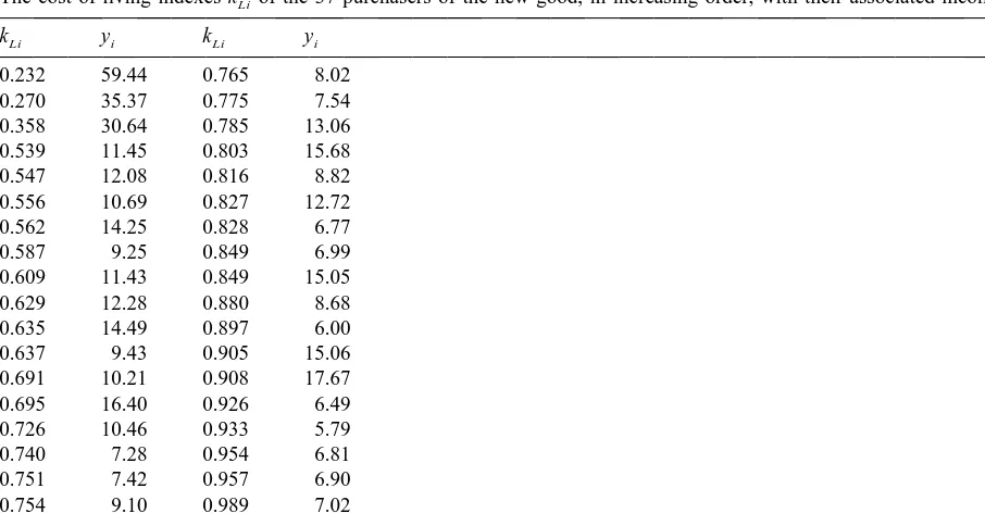
Table 1
a
The cost-of-living indexes kLiof the 37 purchasers of the new good, in increasing order, with their associated incomes yi
kLi yi kLi yi
For comparison, the average individual income in the population of 400 is 4.06, the maximum individual income is 59.44, and the minimum is 0.36. The cost-of-living index equals 1 for all individuals in this population other than the above 37 above.
4. Example: introduction of a new good
I suppose there is one variety in the reference period, with a second introduced in the comparison
r c r c c c
period. I set p15p15x15x151, p255, and x252, so that the new variety has both higher quality and higher price than the existing variety. Following Hicks (1940), I pretend that the second variety is
r r
available in the reference period at a price so high that no individual purchases it; any p , x
s
2 2d
satisfying this restriction produces the following results: (i) only 37 of the M5400 individuals purchase the new good; (ii) each of the remaining 363 individuals has a Laspeyres–Konus index equal to 1, the median; (iii) the ordinary mean of the individual indexes equals 0.975; (iv) the income-share-weighted mean equals 0.892. Table 1 shows the 37 individual indexes less than unity, with their associated incomes. Clearly, a small number of high-income people enjoyed large benefits from the new good; whether this is well-represented by saying the population as a whole enjoyed a 10% fall in the cost of living is debatable.5. Example: quality improvement in an existing good
Here I assume that only one variety is available in both the reference and comparison periods. To
r c r c
225 in the reference period to 88 in the comparison period; (ii) the median Laspeyres–Konus index equals 1; (iii) the ordinary mean of the individual indexes equals 1.15; (iv) the income-share-weighted mean equals 0.909. Thus, depending on how you weight the individual cost-of-living indexes, the aggregate cost of living can increase or decrease. The existence of individuals who are worse off makes this possible, and such individuals can exist if the old version of an improved good is no longer available. Individuals who choose not to buy an improved good because of an accompanying price increase are worse off to exactly the same degree as if the price rise was unaccompanied by a quality improvement.
6. Conclusion
The aggregate-data Laspeyres price index is used by many government statistical agencies to summarize price movements in markets for expensive discrete goods, such as houses and cars. The examples in this note, combined with the fact that the aggregate Laspeyres price index equals the household-expenditure-share weighted average of the individual household Laspeyres indexes, suggest that the welfare implications of quality change and new goods cannot be fully understood by looking at the aggregate index alone. This is so, even when the aggregate index is evaluated using prices that have been adjusted to account for changed quality and availability. It may therefore be useful, feasibility permitting, for statistical agencies to supplement their aggregate indexes with estimates of the corresponding distributions of individual indexes.
Acknowledgements
I thank Dennis Fixler, Pat Jackman, Rob McClelland, Brent Moulton, and Toni Whited for helpful comments. Any opinions expressed in this paper are my own and do not constitute policy of the U.S. Bureau of Labor Statistics.
References
Berry, S., Levinsohn, J., Pakes, A., 1995. Automobile prices in market equilibrium. Econometrica 63, 841–890. Hausman, J., 1997. Cellular telephone, new products and the CPI, mimeo, MIT.
Hicks, J., 1940. The valuation of the social income. Economica 7, 105–124.