Vol. 43 (2000) 447–470
Economic motives and professional norms:
the case of general medical practice
Tor Iversen
∗, Hilde Lurås
Health Economics Research Programme at the University of Oslo (HERO), Center for Health Administration, The National Hospital, N-0027 Oslo, Norway
Received 10 June 1998; received in revised form 9 February 2000; accepted 23 February 2000
Abstract
Professional norms are supposed to have a central role in the allocation of resources when consumers have inferior information about the characteristics of products. We argue that economic motives are nevertheless important to resource allocation when professional opinions differ. The argument is illustrated with an example from medical care. We find that physicians who experience a shortage of patients have higher income, longer and more frequent consultations and more laboratory tests per listed person than their unconstrained colleagues. © 2000 Elsevier Science B.V. All rights reserved.
JEL classification: H42; I11; I18
Keywords: Economic motives; Professional norms; Capitation; General practice; Patient shortage; Service provision
1. Introduction
When consumers have little knowledge about characteristics of products, professional norms are often assumed to play a central role in the allocation of resources. For instance, Arrow (1963) argued that this is a major function of professional norms for medical doctors. An interesting question is whether personal economic motives are then absent. In this paper, we argue that economic motives are important to resource allocation when professional opinions differ. Our example is from medical care when it is not clear what constitutes the right treatment for a patient.
The focus is on demand creation among general practitioners (GPs). We shall examine whether GPs who experience a shortage of patients (rationing) provide more services to
∗Corresponding author. Tel.:+47-23-07-53-00; fax:+47-23-07-53-10.
E-mail addresses: [email protected] (T. Iversen), [email protected] (H. Lurås).
each of their patients than their unrationed colleagues. Our study employs data from the Norwegian capitation experiment initiated by the central government in the early 1990s.1 Due to the experiment, the payment system for GPs was also changed. In the previous system, most GPs were self-employed contract physicians while the rest were municipal employees on a fixed salary. In the new remuneration system, a GP’s income consists of a per capita component per listed person and a fee-per-item component. Compared with the remuneration system of the contract physician in the previous system, the municipal grant and some fees were replaced by the capitation component.2
All GPs in four municipalities participated in the experiment, and all inhabitants in these municipalities were listed by a GP. We have ex ante information about the number of persons that each GP would like to have on his list at the start of the experiment. A GP’s preferred list size reveals information about a physician’s preferred practice style and his preferred workload. By comparing preferred list size ex ante and actual list size during the experimental period we can distinguish empirically between those GPs who experience a shortage of patients (rationing) and those who do not.
Our micro data on individual GPs’ preferred and actual number of patients improve on previous studies by introducing the possibility of patient constraints at the individual practice level.3 We find that GPs who experience a shortage of patients provide more services to their patients and use all kinds of fees more frequently than their unconstrained colleagues. An important policy implication of our study is then that GPs’ choice of service provision seems to depend on economic motives.
In the health economics literature, considerable attention is devoted to whether physi-cians, in order to generate income, induce demand for their own services.4 Many authors are critical as to whether empirical studies in fact have managed to distinguish effects of supplier-induced demand from effects of better access. Dranove and Wehner (1994) point out two factors that may cause the problem of identification: the first stage regression is not identified and border crossing of patients is not adequately addressed. The first factor stems from the fact that the number of physicians in an area may not be exogenous, but influenced by the volume of health services provided. Two-stage least squares estimation is therefore applied. The first stage identifies a physician supply equation, and ideally includes variables that are related to physician supply and unrelated to the demand for physician services. Dra-nove and Wehner (1994) question whether the variables used are able to identify the first stage regression. In our study, this problem is solved, since we have data describing the individual GP’s actual number of patients compared with his preferred number. Variation in GP density at the municipal level is taken into account by introducing dummy variables. Since patients are listed with a GP practising in the municipality where they are residents, border crossing of patients is not a problem in our analysis.
1The system with capitation in general practice has long since been established in countries like Denmark, the
Netherlands and the UK.
2The fee-per-item component from the National Insurance Scheme and from patient charges is paid according
to a fixed fee schedule. The fees are decided in centralised negotiations between the physicians’ union and the state.
3Scott and Shiell (1997a,b) provide a review of the literature and recent empirical results.
4See, for instance, Evans (1974), Feldman and Sloan (1988), Phelps (1986), Rice and Labelle (1989), Hughes
In Section 2, we present a model that determines a physician’s optimal number of patients and intensity of service provision in the rationed and in the unrationed case. A detailed de-scription of our data can be found in Section 3. Section 4 describes the estimation procedure and the results of the empirical analysis. Section 5 provides concluding remarks that include suggestions for further studies.
2. A GP’s optimal number of patients and intensity of service provision
In this section, we model the effect of economic constraints on a GP’s optimal practice profile in a mixed capitation and fee-per-item system. The practice profile is characterised by the number of patients the GP takes responsibility for, and the volume and composition of services he provides to his patients. We shall assume that the marginal product of health care on health is a declining function of the volume of services provided. This relation may, for instance, be explained by the fact that the health effect of an initial consultation with a GP is usually greater than the health effect of the following check-ups. Providing too many health services may even contribute negatively to a patient’s health on the margin. Too many diagnostic tests increase the probability of false positive results and excessive medication may have considerable adverse effects.
For a number of GP consultations it is not clear what constitutes ‘the right medical treatment’. The reason may be heterogeneity among patients with similar symptoms or diagnoses. But it may also be due to different opinions among physicians regarding the optimal volume of health services with respect to a patient’s health. For instance, views among physicians may differ with respect to how often a patient with diabetes or a patient with hypertension should be called for check-ups. Views may also differ on whether a GP who prescribes antibiotics to a patient should call in the patient for a follow-up consultation next week, or ask the patient to contact him if he feels worse. The intensity of service provision will on average be higher in the first case than in the second.5 It is also well documented that referral rates of GPs vary more than can be explained by the composition of patients. For our purpose, an interesting consequence of the lack of medical standards is that several practice profiles are all regarded as equally satisfactory from a professional point of view.6
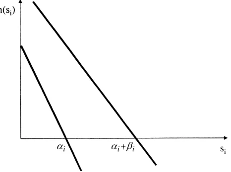
Fig. 1 describes the range of professional opinions about the relationship between a health service, si, and its marginal health effect, h(si). The downward sloping line to the left
expresses the most pessimistic view, while the downward sloping line to the right expresses the most optimistic view about the marginal effect of health services. The figure describes an interval, [αi,αi+βi], where the marginal effect of health services is not documented
to be different from zero.7 Medical practice variation and the lack of medical standards are arguments for the existence of this interval. Other things equal, professional consensus about treatment profiles contributes to narrowing the interval.
5A thoughtful discussion of the various aspects of uncertainty in knowledge about the efficacy of medical
interventions is given by Phelps (1992).
6For an introduction to the literature on medical practice variation, see Andersen and Mooney (1990). 7In the health economics literature this interval is often referred to as ‘flat of the curve medicine’, see for instance
Fig. 1. The range of professional opinions about the marginal effect of health services.
We denote the number of health services in excess ofαi as ki. To simplify the
anal-ysis, we shall assume only two health services. Furthermore, αi is assumed to depend
on kj, (i6=j), such that αi=αi(kj). For instance, if service no. 1 is consultations in the
physician’s office and service no. 2 is consultations by telephone, it seems reasonable that
∂α1(k2)/∂k2<0. On the other hand, if service no. 1 is medication requiring monitoring, we
may have∂α1(k2)/∂k2>0.
The value ofαiandβimay vary between groups of patients. The number of episodes of
illness during a certain period, as well as the marginal benefit from health services during an episode of illness, may differ. For instance, elderly persons with chronic diseases may need more health services to stay healthy than young people. We introduce a parameter,θ, to account for variation in need according to patient group.θis considered to be exogenous to the individual GP.8 We then haveαi=αi(θ, kj) andβi=βi(θ), where the partial derivatives
with respect to θ are positive. We shall assume that the distribution of θ describes the physician’s population of patients.θhas the probability density function f(θ), whereθ∈(0, ∞). F(θ) is the cumulative distribution function. We shall assume that the physician can influence the number of patients (n) he takes care off. The distribution of patients according to groups is, however, assumed to be exogenous to the physician.
We assume that a physician decides the quantity of health services provided to each of his patients.9 We further assume that a physician has lexicographic preferences concerning
his patients’ health and his own income and leisure. This assumption implies that a patient’s health is never balanced against the GP’s income or leisure. Health services are then provided until the marginal health effect is equal to zero. This assumption simplifies the formal reasoning considerably and it is also in accordance with the medical profession’s own
8Since we have a one-period model, it is reasonable to assume thatθis exogenous. In a two-period modelθin
this period may, however, depend on the volume of health services provided in the previous period.
9The number of patient-initiated contacts is assumed to be included inα
assertion. A relaxation of this assumption would imply that the effect of economic incentives is strengthened.
We assume a quasilinear objective function formulated in monetary terms as V=c+v(l), where c is consumption (all income is consumed) and l is leisure.v(l) is assumed to be strictly concave withv′(l)>0. The physician’s decision problem may now formally be expressed as
maxc
wherewis a fixed salary or practice allowance, q is a capitation payment per person on the physician’s list of patients, piis the fee per item of health service (or equivalently, a fee for
service) no. i (i=1, 2),10 tiis the time input of providing health service no. i, T is the total
time endowment andn¯is a constraint on the number of patients. All of these variables are assumed to be exogenous to the physician.11 (i) and (ii) say that the number of services provided to a patient must be within the interval where the marginal effect of services on health is not documented to be different from zero. (iii) says that the number of patients is positive, but physicians may experience a shortage of patients. We shall only consider cases where n is positive.
The maximisation problem is analysed by means of concave programming.12 Because the empirical part of the paper employs data from a mixed capitation and fee-per-item system, we shall concentrate on the model’s predictions under this system.13 When q>0,
p1>0, p2>0,w=0 and ‘a’ is the net fee per time unit of service no. 2 relative to service no.
1 we have the following results.
In a combined capitation and fee-per-item system:
• The minimum volume of both services is provided when the income per time unit of providing service no. 1 is equal to the income per time unit of providing service no. 2 (a=1) and in an interval around a=1.
• Outside this interval: when the income per time unit of providing service no. 1 is larger (smaller) than the income per time unit of providing service no. 2, the maximum (mini-mum) volume of service no. 1 and the minimum (maxi(mini-mum) volume of service no. 2 are provided.
10p
imay be interpreted as a net fee, i.e. the gross fee minus the physician’s costs for employed personnel and
other inputs except own time.
11Assuming t
ito be exogenous is not quite realistic, but it simplifies the analysis and plays no substantial role
for our conclusions.
12Details can be found in Appendix A.
• When a shortage of patients occurs, even the less profitable service may be provided in excess of the minimum volume.
The intuition behind the result is: in a pure fee-per-item system the relative fee per time unit (a) determines the optimal number of each service. If a6=1, the least paid service will be provided at the minimum volume (ki=0), while the best paid service will be provided
at the maximum volume (kj=βj). On the other hand, in a pure capitation system, where
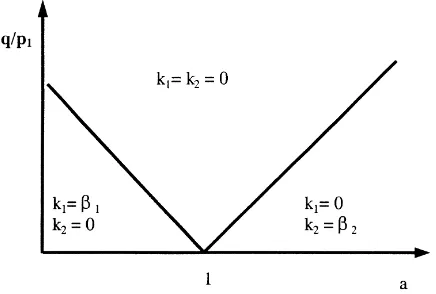
the list of patients is the only income-generating component for the GP, the volume of both services is chosen equal to the lower constraint. In a combined payment system, the size of the capitation component relative to the fee-for-service component determines the optimal service provision. Even if a6=1, extra provision of the best paid service has an opportunity cost of reduced income from capitation. If this opportunity cost is ‘large enough’ relative to the fee-for-service component, the provision of both services is kept to the minimum (k1=k2=0). With a shortage of patients, the opportunity cost declines and hence, the service
provision is likely to increase. The solution is shown in Fig. 2.
In Appendix A, it is shown that k1,k2and n are homogenous of degree zero in p1, p2
and q. In Fig. 2, the curve that illustrates the margin between the k1=k2=0 and k1=β1,
k2=0 is downward sloping because a decline in ‘a’ makes it more profitable to increase the
provision of service no. 1. Hence, an increase in q is necessary to restore the indifference. By similar reasoning, it follows that the curve showing the margin between k1=k2=0 and
k1=0, k2=β2is upward sloping.
Fig. 2 also illustrates that the introduction of a capitation component implies that k1=k2=0
even when a6=1 is in the intervala,a¯. The result illustrates a point emphasised by Newhouse (1992, 1996); because of the practical difficulties of fine-tuning a single payment component, a mixture of payment components is more robust in order to achieve health policy objectives. Let us finally consider the feasible solutions when there is a shortage of patients, i.e. n= ¯n. Letµbe the Lagrange parameter related to the third constraint in (1), expressing the increase in utility of a marginal loosening of the constraint, i.e. a marginal increase in the number of patients. Hence,µ>0 when n= ¯n. The magnitude ofµrelative to the per capita component
q plays an important role in the constrained case. Ifµ<q, the increase in utility is less
than the capitation fee. This means that the marginal utility from increasing the volume of services with the optimal composition of services is negative: the marginal value of leisure is larger than the income from marginal service provision. Then, the number of services per patient in the constrained case is equal to the number of services in the unconstrained case. Ifµ>q, the income from marginal service provision with an optimal composition of services is larger than the marginal value of leisure. The number of services per patient in the constrained case is then larger than the number of services in the unconstrained case. The most profitable service is certainly offered at the maximum level, and if the shortage of patients hurts enough, even the less profitable service may be offered in excess of the minimum volume. We are not able to distinguish empirically between GPs according to the relation betweenµand q. However, ifµ>q for at least one GP in our sample, we will find an effect of rationing on the volume of services provided. In Appendix B, we show that if
µ>q, the maximum number of both services is provided even with a=1. The interpretation ofµ=q should now be obvious.
From the model’s result the following testable hypotheses follow directly.
• A GP’s income from fees per listed person is expected to be higher in the constrained case (a shortage of patients) than in the unconstrained case, because more services per person are expected to be provided.
• If the constraint hurts enough, even the less profitable services are expected to be provided in excess of the minimum volume in the constrained case.
We shall also take into account an effect of patient composition that follows directly from one of the model’s assumptions.
• A GP’s income per listed person increases when the composition of the list shifts towards a population with a greater need for health services (a negative shift in F(θ)).
3. Description of the data
Data from the Norwegian capitation experiment are applied. Annual data for each physician’s practice income were collected in 1994 and 1995. The total fee-for-service component consists of the payment from the National Insurance Scheme and from patient charges. This aggregate is used as an indicator of the total volume of services provided in a GP’s practice during 1 year (INPERCAP). Data describing the composition of the fee-for-service component were collected in two representative periods of 14 days, one in March 1994 and one in March 1995.
The number of ordinary consultations (CONSULTS) and the number of laboratory fees (# LABS) per listed person are used as indicators of the best-paid services. The fee schedule also contains a fee that depends on the duration of the consultation. If the consultation lasts more than 20 min, the GP receives an additional NOK 56 per started 15 min. The ordinary fee per consultation with a duration of less than 20 min is NOK 78. Hence, the fee depending on the consultation duration is likely to be less profitable than the ordinary consultation fee. The number of consultations per listed person when this fee is used (DURATION) is an indicator of the frequency of providing the less profitable services.
outliers.14 Our income data then consist of 218 observations, while the service provision data include 183 observations.
According to Fig. 2, both of the services are provided at a minimum level if the capitation fee is high compared with the fee for service. In our data the capitation fee is NOK 236. Hence, the capitation fee is about four times the fee for long consultations. We suspect this difference to be large enough to encourage k1=k2=0 in the unconstrained optimum. An
example illustrates our prediction: assume that an average ordinary consultation lasts 15 min and an average long consultation lasts 30 min. An additional listed patient has on average two consultations per year. One of these consultations is assumed to be a consultation of long duration. The income per hour of providing more consultations to the present list of patients is then NOK((78×60)/15))=NOK 312, while the expected income per hour of adding one patient to the list is NOK((236+78+78+56)×60)/45=NOK 597. Hence, it is more profitable to provide few services to a long list of patients than to provide many services to a short list of patients. Hence, we expect that k1=k2=0 in the unconstrained
optimum and, accordingly, that the whole range of services is expected to increase when a shortage of patients occurs.
One important conclusion from our theoretical model is that physicians who experience a shortage of patients have a more service intensive practice style than their unconstrained colleagues. Before the experiment started, all the participating GPs were asked to specify the number of persons they would like to have on their individual lists (PRELISTSIZE). It is important to note that a GP both takes account of his own characteristics, such as family situation and medical experience, and his own practice style when he expresses his preferred list size. For instance, one GP may wish to work 10 h each day, another prefers a part-time job, one prefers short consultations and yet another prefers to use considerable time on a patient during the consultation. It follows that the preferred number of persons on the list is likely to vary substantially between GPs. For each GP we compare preferred list size and actual list size and obtain an indicator of individual patient constraints. Hence, the absolute size of the lists and the reason why the size varies between GPs are not an issue in this study. Two dummy variables indicate whether GPs are rationed. The dummy variable RA-TION A is equal to one for those physicians who had a smaller list than they wanted in period one and experienced a net increase in the number of patients from period one to period two. The second dummy variable, RATION B, is equal to one for those physicians who had a smaller list than they wanted in period one and experienced a constant or a declining number of patients from period one to period two. Our data then consist of three groups of GPs according to rationing status: unrationed, lightly rationed (RATION A) and strongly rationed (RATION B) GPs. We predict that constrained GPs consider an increased number of patients in period two as a signal of a less severe constraint. Accordingly, it is optimal for them to have a less aggressive practice style than their colleagues experiencing a shortage of patients in the first period and a constant or a declining list of patients in the second period. Hence, the effect of both light and strong rationing is expected to be positive, and the effect of the former is expected to be weaker than the effect of the latter.
14Their registered income per listed patient differed substantially between 1994 and 1995. We therefore suspect
The distribution of patients according to age and gender is expected to influence the volume of services provided. It is well known from various studies that females have more frequent consultations than men and that the elderly have more frequent consultations than younger (disregarding the infant age) people (Elstad, 1991). As an indicator of the patient load we used the female proportion of patients (PROPFEM) and the proportion of patients aged 70 and older (PROPOLD). These data were collected annually. Female physicians seem to have a practice style that differs from their male colleagues (Langwell, 1982). Kristiansen and Mooney (1993) found that on average female GPs had longer consultations than male GPs. In the analysis we take account of the physician’s gender (FEMALE). All the GPs in our set of data are self-employed. Prior to the capitation experiment, however, some of the physicians were employed by the municipality on a fixed salary contract. It follows that they were unfamiliar with the fee schedule compared with their privately practising colleagues. In the transition period, the income from fees may therefore underestimate their volume of service provision. We therefore introduced a dummy variable to account for the physician’s employment status before the experiment (SALARIED).
From Table 1 we see that the mean annual income from fees and patient charges per person listed for the whole sample of GPs was NOK 237. On average, 51 percent of the persons on the individual lists were women and nearly 10 percent were aged 70 and older. Thirty-seven percent of the physicians included were salaried community physicians prior to the experiment and 26 percent of the physicians were female. During the 14 days of registration the GPs on average provided 0.07 consultations, 0.07 laboratory tests and used the duration-dependent fee 0.02 times per listed person. Calculated on an annual basis (multiplied by 26), our figures correspond to 1.9 consultations per person per year.
Almost 40 percent of the GPs were lightly rationed and 26 percent experienced strong rationing. Hence, almost 66 percent of the physicians experienced a smaller list in period 1 than they preferred when the experiment was initiated. As seen from Table 1, the strongly rationed group annually earns NOK 50 more per listed person from the fee-for-service component than their unrationed colleagues. On average, both categories of rationed GPs provide more consultations, use the duration-dependent fee to a greater extent and provide more laboratory tests per listed person than their unconstrained colleagues.
4. Estimation and results
Because there are two periods of observations of each GP, and each GP belongs to a specific municipality,15 our data have a hierarchical structure. Demographic and cultural characteristics and the organisation of primary care at the municipal level are likely to influence the practice styles and hence, our observations of GPs at the municipal level. There is also reason to believe that the practice style has individual characteristics, making an observation in one period dependent on the observation in the other period for identical GPs. The implication of a hierarchical structure of the data is that the assumption of independent
15In the annual income data there are 218 observations (level 1) of 109 GPs (level 2) from four municipalities
error terms in OLS is not valid. We make use of an estimation procedure that accounts for the multilevel structure and the possible clustering of data (Goldstein, 1995). This approach corresponds to the one reviewed by Rice and Jones (1997) and used by Scott and Shiell (1997a,b). We assume
yijk=a+(b+wjk)xijk+vjk+uijk
where yij kis the dependent variable with a subscript indicating observation no. i of GP no.
j in municipality no. k, and xij kis the independent variable with a similar subscript. uij kis
the stochastic error term at level 1 (observation) andvjkis the error term at level 2 (GP).
wjkis the random coefficient of the slope associated with the explanatory variable xij k.16
Since level 3 in our data has only four possible values, we choose to include the mu-nicipalities as fixed effects17 (we therefore from now on suppress the subscript k). This formulation implies that the ‘constant term’ is considered to have a random element at each of the two levels. Since our data set consists of two observations of each unit, the similarity with panel data analysis is obvious.
We make the following assumptions regarding the distribution of the stochastic error terms of each of the two levels.18
E(uij)=0, var(uij)=σ2, covar(uij, ukl)=0 for i6=k, j 6=l E(vj)=0, var(vj)=σv2, covar(uij, vj)=0
E(wj)=0, var(wj)=σw2, covar(uij, wj)=0 and covar(vj, wj)=σvw
The total variance is then
var(yij|a, b, xij)=var(vj +wjxij+uij)=σv2+2σvwxij+σw2xij2+σ2
and the covariance between two observations of the same physician is
cov(vj+u1j, vj+u2j)=cov(vj, vj)=σv2
since level 1 residuals are assumed to be independent.
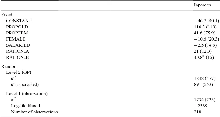
When estimating the model we choose the random structure that maximises the likelihood of the model. The estimation procedure applied is the iterative GLS as modelled in the statistical software MLn. We first estimated the effect of rationing on the total income per listed person. The results of the estimation are shown in Table 2.
We observe that the estimated variance at level two is considerable, indicating a correla-tion between a GP’s practice style in the two periods. In the language of Fig. 1 in Seccorrela-tion
16In the analysis of the composition of the GP’s income (Table 3) we did not include a random coefficient:w
jk=0.
17In the first step of the regression we estimated the effect on the dependent variable of the municipalities. We
corrected the dependent variable for this effect, and in the second step of the regression we used this corrected dependent variable.
18Since there are two consecutive observations of each GP, one would suspect autocorrelation, i.e.
covar(u1j,u2j)6=0. We have run a regression with û1jas an independent variable and û2jas a dependent
Table 2
The estimated effect of a shortage of patients on income per listed person (INPERCAP) (standard deviations in parenthesis)
Inpercap Fixed
CONSTANT −46.7 (40.1)
PROPOLD 116.3 (110)
PROPFEM 41.6 (75.9)
FEMALE −10.6 (20.3)
SALARIED −2.5 (14.9)
RATION A 21 (12.9)
RATION B 40.8∗(15)
Random Level 2 (GP)
σv2 1848 (477)
σ(v, salaried) 891 (553)
Level 1 (observation)
σ2 1734 (235)
Log-likelihood −2389
Number of observations 218
∗This indicates that the estimated parameter is significantly different from zero at the 5 percent level with a
two-tailed test.
2, the implication of the large unexplained variance of practice style is that the interval (αi,
αi+βi) is large. We have assumed that the error term at level two is correlated with the
vari-able SALARIED because the log-likelihood with this variance–covariance structure was significantly higher than the log-likelihood when a simple random structure was applied.
The results indicate a positive effect of rationing for both groups of rationed GPs. The effect of strong rationing is significant. The results imply that a GP who experiences a light shortage of patients is expected to have 9 percent higher income from fees per patient than his unrationed colleagues. A GP who experiences a severe shortage of patients is expected to have 17 percent higher income per patient than the group of unrationed physicians. Hence, more severe rationing means higher income per listed person than less severe rationing. If we compare these results with the average list size for the three groups of GPs, we will note that although the group of strongly rationed GPs had on average 211 more persons on their list than the lightly rationed group, they earned more per listed person per year. This clearly illustrates the effect of physicians’ preferences for income relative to leisure on their practice style.
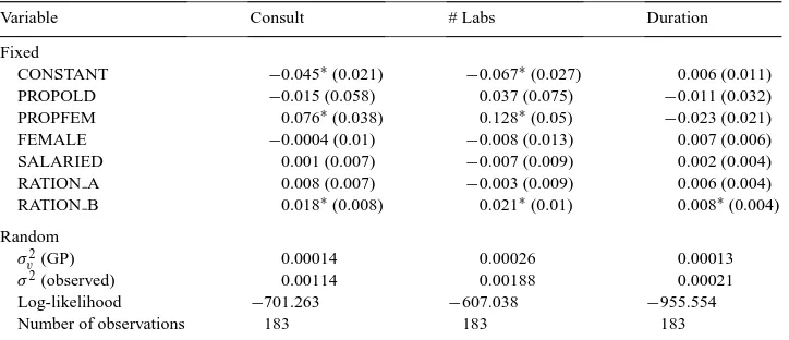
Table 3
The estimated effect of rationing on consultations per listed person (CONSULT), on consultations that have a long duration (DURATION) and the number of laboratory fees used (# LABS) per listed person (standard deviations in parenthesis)
Variable Consult # Labs Duration
Fixed
CONSTANT −0.045∗(0.021) −0.067∗(0.027) 0.006 (0.011)
PROPOLD −0.015 (0.058) 0.037 (0.075) −0.011 (0.032)
PROPFEM 0.076∗(0.038) 0.128∗(0.05) −0.023 (0.021)
FEMALE −0.0004 (0.01) −0.008 (0.013) 0.007 (0.006)
SALARIED 0.001 (0.007) −0.007 (0.009) 0.002 (0.004)
RATION A 0.008 (0.007) −0.003 (0.009) 0.006 (0.004)
RATION B 0.018∗(0.008) 0.021∗(0.01) 0.008∗(0.004)
Random
σv2(GP) 0.00014 0.00026 0.00013
σ2(observed) 0.00114 0.00188 0.00021
Log-likelihood −701.263 −607.038 −955.554
Number of observations 183 183 183
∗This indicates that the estimated parameter is significantly different from zero at the 5 percent level with a
two-tailed test.
Our main conclusion so far is that GPs experiencing constraints regarding the number of patients provided more services to each patient than unconstrained GPs. One might claim that this result occurs because the unconstrained GPs experience too many patients on their list19 and hence they provide fewer services to their patients than their optimal level. In supplementary analyses we included dummies to take account of the practice style for GPs who had more patients than they preferred on their list. We still found a positive significant effect of strong rationing on GPs’ income. This effect is larger in absolute value than the negative and not significant effect of having more patients than the preferred number.
An interesting question is now whether we can trace this higher income from fees per listed person to any specific component of the fee schedule.
The effects on the number of consultations per listed person are shown in the first column of Table 3. Again, both of the rationing dummies are positive and we find that more severe rationing implies an increase in the number of consultations per person. The effect of more severe rationing is significant. We may then conclude that the number of consultations per person is part of the explanation behind the result of higher total income per listed person for GPs experiencing a shortage of patients.
In the second column we have examined the effect on the use of fees related to laboratory tests. Again, a significantly positive effect of rationing was found in the strongly rationed group. This group of physicians will on average provide 29 percent more laboratory tests per listed person than the group of unconstrained GPs. We conclude that more frequent use of laboratory fees is another reason why rationed GPs had higher total income per listed person.
We use the number of duration-dependent fees per listed person as an indicator of the frequency of providing a less profitable service. The result of this analysis is shown in the third column of Table 3. The effect of rationing has the expected sign: on average a constrained GP uses the duration-dependent fee 25 and 33 percent, respectively, more per person than an unconstrained GP.
5. Concluding remarks
In the theoretical section of this paper, we studied the effect of a shortage of patients on a GP’s practice profile in a mixed capitation and fee-for-service payment system. A GP’s preferred list size reveals information about his preferred practice style and preferred workload. When a GP’s actual list size deviates from the preferred one, we expect him to have a practice style that deviates from his unconstrained optimal choice. We predicted that the fee-for-service component in the payment system motivates physicians who experience a shortage of patients to have a more service-intensive practice style than their unconstrained colleagues. We also predicted that a GP experiencing a shortage of patients even provides the least profitable services in excess of the minimum volume.
Data from the Norwegian capitation experiment were used to test the hypothesis. We applied an estimation procedure that took account of the hierarchical structure of the data. The results show that constrained physicians have higher incomes from fees per listed person than unconstrained GPs. In addition, the use of the various fees is in accordance with the predictions from the theoretical model. GPs experiencing constraints on the number of patients provided the best-paid services — ordinary consultations and laboratory tests-more often than unconstrained GPs. They also provided the less profitable service — the long consultation-more often than the minimum volume.
Our modelling of physician behaviour may be interpreted as a special case of monopolistic competition as analysed in the classic work of Chamberlin (1933). Under monopolistic competition each firm has individual characteristics that result in a demand curve for each firm’s products. The individual demand curves are less steep than the market demand curve, but not horizontal, as in the perfect competition case. Each firm is able to shift the individual demand curve by means of advertising and other types of activities that add to its selling costs. In our application, the demand for enrolment on a GP’s list is a function of the GP’s individual characteristics. This demand may deviate from the GP’s supply of list openings (preferred list size) determined by the condition that income per unit of time from an additional patient equals the marginal cost in terms of lost leisure. If the demand is less than the supply, the GP is rationed. Since the public insurer sets all prices, price competition is ruled out. Individual characteristics of GPs are considered exogenous. The demand side therefore determines the actual number of patients on each GP’s list. The rationed GP may influence the average income generated by each patient by adjusting the number of services provided. This adjustment is costly since there is a positive shift in the marginal cost curve because each patient now requires more of the GP’s time.
list of patients and fewer services to each of the patients. That each patient receives less care in the GP’s unconstrained optimum than in the constrained optimum contradicts the notion that altruism is an important motive behind the provision of extra services.
We assumed that GPs never balance a patient’s health against own income. From a normative point of view, the model then seems to imply that a pure capitation system is socially optimal, since only the necessary volume of services per patient is then provided. One may, however, claim that a pure capitation system leads to underprovision, since GPs in fact balance a patient’s health against own income. Our study has no ambition of determining whether this is true. Our aim is limited to studying whether a GP’s practice profile is influenced by economic motives. A positive answer to this question is a necessary condition for the workings of economic incentives. Finding a payment system that encourages GPs to deliver the socially optimal volume of services requires additional information on GPs’, patients’ and insurers’ objective functions.
An implication of our study of relevance to health policy is that GPs’ choice of service provision seems to depend on economic motives. This result is probably not surprising to economists, but still controversial among health care workers and politicians. For instance, the entire focus in Norway seems to be on the shortage of GPs, while our study emphasises that organisation and payment system seem to influence perceptions of GP shortage. A shortage of GPs in one system may well be transformed into a shortage of patients in another system, which in turn may influence the actual service provision to patients. For instance, a practice allowance component is paid out independent of the number of persons a GP takes care of, while a capitation component will encourage GPs to take care of a large number of patients. When a capitation component replaces a practice allowance component, this may imply a switch from a situation with a shortage of GPs to a situation with a shortage of patients. When the payment system also consists of a fee-for-service component, a rationed GP, according to our results, is likely to compensate for the income loss by providing more services to his patients. This may well happen when a capitation system is introduced, as in Norway from the year 2001.
Acknowledgements
The authors are grateful to the participants, especially Lise Rochaix, at the Sixth European Workshop on Econometrics and Health Economics in Lisbon 10–13 September 1997 for constructive criticism of a previous version of the paper. Suggestions from Sverre Kittelsen, Tor J. Klette and Steinar Strøm have contributed to improving the paper. Three anonymous referees and the Editor have contributed substantially to improving the article. Financial support from the Norwegian Ministry of Health and Social Affairs and the Research Council of Norway is acknowledged.
Appendix A. Derivation of the results in Section 2
L(k1, k2, n)=w+qn+n
A necessary and sufficient condition for ki≥0 (i=1, 2) and n>0 to solve the problem is
that there are non-negativeλ1,λ2andµsuch that
∂L(k1, k2, n)
The explicit expressions for∂L/∂kiand∂L/∂n are found from the partial derivatives of the
Lagrangian
is the expected (ex ante) effect of having an additional patient for the provision of service no. i (i=1, 2).
Assumingti+tjEki(αj) > 0 (i, j =1,2), implying that the direct effects are greater
than the indirect effects, we can express (A.2) as
v′(l)≥ (p1/t1)[t1+at2Ek1(α2)]−(λ1/n)
t1+t2Ek1(α2)
v′(l)≥ (p1/t1)[at2+t1Ek2(α1)]−(λ2/n)
t2+t1Ek2(α1)
v′(l)=q+(p1/t1)[t1En(α1+k1)+at2En(α2+k2)]−µ
t1+En(α1+k1)+t2En(α2+k2)
(A.3)
Consider first the alternatives without constraint on the number of patients, i.e. n<n¯and henceµ=0. Assume then 0<k1<β1and 0<k2<β2, and hence,λ1=λ2=0. From (A.1) we
then have
q+(p1/t1)[t1En(α1+k1)+at2En(α2+k2)]
t1En(α1+k1)+t2En(α2+k2)
=(p1/t1)[t1+at2Ek1(α2)]
t1+t2Ek1(α2)
(A.4a)
q+(p1/t1)[t1En(α1+k1)+at2En(α2+k2)]
t1En(α1+k1)+t2En(α2+k2)
=(p1/t1)[at2+t1Ek2(α1)]
t2+t1Ek2(α1)
(A.4b)
For a=1 we see that the left-hand side of both (A.4a) and (A.4b) is larger than the right-hand side, which contradicts the equality sign. For a<1 the right-hand side of (A.4b) is smaller than the left-hand side, which contradicts the equality sign. For a>1 the right-hand side of (A.4a) is smaller than the left-hand side. Hence, for n<n¯, 0<k1<β1and 0<k2<β2is not a feasible solution.
Consider next k1=k2=0, and hence,λ1=λ2=0. From (A.1) we then have q+(p1/t1)[t1En(α1+k1)+at2En(α2+k2)]
t1En(α1+k1)+t2En(α2+k2)
>(p1/t1)[t1+at2Ek1(α2)] t1+t2Ek1(α2)
(A.5a)
q+(p1/t1)[t1En(α1+k1)+at2En(α2+k2)] t1En(α1+k1)+t2En(α2+k2)
>(p1/t1)[at2+t1Ek2(α1)] t2+t1Ek2(α1)
(A.5b)
The left-hand side of both (A.5a) and (A.5b) is increasing in ‘a’ 20 and q. The right-hand side of (A.5a) is decreasing in ‘a’, while the right-hand side of (A.5b) is increasing in ‘a’, and increasing more rapidly with ‘a’ than the left-hand side. (A.5a) and (A.5b) are both fulfilled for a=1. It then follows that there is an intervala<a<a¯ around a=1, where the inequality signs are fulfilled and hence, k1=k2=0. This interval increases with q.
By means of similar reasoning, we can show that k1=0 and k2=β2are possible if ‘a’ is
large enough and k1=β1and k2=0 are possible if ‘a’ is small enough.
Appendix B. Optimal service provision under alternative payment systems
We isolate the effect of each of the payment components.
20An increase in ‘a’ with p
B.1. Fixed salary:w>0, q=p1=p2=0
In this case we have from (A.3) thatv′(l)=0, which implies l≈T and is obviously not feasible. Within our line of thought this is not possible without a constraint on leisure in the fixed salary case. The intuition behind this result is straightforward: since there is no community responsibility in the objective function, the physician wants as few patients as possible in order to increase his leisure time. Therefore the leisure constraint is effective. The physician is indifferent between the various feasible combinations of k and n. We shall not pursue this case further, since a fixed salary is not part of the paper’s empirical section.
B.2. Capitation: q>0,w=p1=p2=0
In this case we have
Result B.1: with capitation the number of both services provided to each patient is ex-pected to equal the minimum volume. When the number of patients is an effective constraint, the provision of services per patient is still kept to the minimum level.
With q>0 andw=p1=p2=0, we have from (A.3) v′(l)≥ −(λ1/n)
t1+t2Ek1(α2)
(B.1a)
v′(l)≥ −(λ2/n)
t2+t1Ek2(α1)
(B.1b)
v′(l)= q−µ
t1En(α1+k1)+t2En(α2+k2)
(B.1c)
Let us first consider the unconstrained case whenµ=0 and accordingly 0<n<n¯. Assume 0<k1≤β1and 0<k2≤β2. Then, according to (A.1a), (A.1c) and (A.1d),λ1≥0 andλ2≥0
and (B.1a) and (B.1b) are fulfilled with equality. But this result impliesv′(l)≤0, which is inconsistent withv′(l)>0 according to (B.1c). Hence, we have k1=k2=0.
Next, considerµ>0 and hence,n¯=n. Again, if 0<k1≤β1and 0<k2≤β2, (B.1a) and (B.1b)
are fulfilled with equality andv′(l)≤0, which is inconsistent withv′(l)>0. Hence, also in the case with rationing we have k1=k2=0.
The intuition behind result B.1 is straightforward. Since the list of patients is the only income-generating component, the volume of services is chosen equal to the lower con-straint and the number of patients is determined such that the marginal income is equal to the marginal value of leisure. When the number of patients is an effective constraint, the provision of services per patient is still kept to the minimum, since the monetary compen-sation for giving up leisure for services is equal to zero. Hence in the rationed case, the marginal income from patients is larger than the marginal value of leisure.
We can sum up the possible solutions. • 0<n<n¯, k1=k2=0.
B.3. Fee per item: p1>0, p2>0, q=w=0
In this case we have
Result B.2: with fee per item of services the composition of service provision depends upon the income per time unit of providing service no. 1 relative to service no. 2. If the income per time unit is independent of the type of service provided, the optimal volume of service provision is undetermined within the feasible interval. If the income per time unit of providing service no. 1 is larger (smaller) than the income per time unit of providing service no. 2, the maximum (minimum) volume of service no. 1 and the minimum (maximum) volume of service no. 2 are provided. If there is a shortage of patients, even the less profitable service may be provided in excess of the minimum level. The exact volume of service provision depends upon the strength of the patient constraint.When p1>0, p2>0 and q=w=0,
we have from (A.3)
v′(l)≥ (p1/t1)[t1+at2Ek1(α2)]−(λ1/n)
t1+t2Ek1(α2)
(B.2a)
v′(l)≥ (p1/t1)[at2+t1Ek2(α1)]−(λ2/n)
t2+t1Ek2(α1)
(B.2b)
v′(l)=(p1/t1)[t1En(α1+k1)+at2En(α2+k2)]−µ
t1En(α1+k1)+t2En(α2+k2)
(B.2c)
We consider first the cases where n<n¯ and 0<k1<β1 and 0<k2<β2. Then, according
to (A.1a), (A.1c) and (A.1d),µ=λ1=λ2=0 and (B.2a) and (B.2b) are both fulfilled with
equality. Then, we have
from(B.2a) v′(l)R p1
t1 ⇔a R1 (B.3a)
from(B.2b) v′(l)Rp1 t1
⇔a⋚1 (B.3b)
from(B.2c) v′(l)R p1 t1
⇔a⋚1 (B.3c)
All three conditions can only be fulfilled for a=1.
Consider next that n<n¯ and k1=k2=0. Then, according to (A.1a), (A.1c) and (A.1d), µ=λ1=λ2=0 and (B.2a) and (B.2b) are both fulfilled with inequality. From (B.2a)–(B.2c)
we have
(p1/t1)[t1En(α1+k1)+at2En(α2+k2)] t1En(α1+k1)+t2En(α2+k2)
>(p1/t1)[t1+at2Ek1(α2)] t1+t2Ek1(α2)
(B.4a)
(p1/t1)[t1En(α1+k1)+at2En(α2+k2)]
t1En(α1+k1)+t2En(α2+k2)
>(p1/t1)[at2+t1Ek2(α1)] t2+t1Ek2(α1)
(B.4b)
For a=1 we have shown that (B.4a) and (B.4b) are both fulfilled with equality. The right-hand side of (B.4a) expresses the income per time unit from an increase in k1. The left-hand side
the right-hand side of (B.4a) will be larger than the left-hand side. The reason is that an increase in the number of patients also implies provision of the less well paid service 2. (B.4a) is then not fulfilled. For a>1 the right-hand side of (B.4b) is larger than the left-hand side through similar reasoning. Then, (B.4b) is not fulfilled. Hence, n<n¯and k1=k2=0 is
not a possible solution.
Consider next n<n¯, k1=0 and k2=β2. Then, according to (A.1a), (A.1c) and (A.1d), µ=λ1=0 andλ2>0 and (B.2a) is fulfilled with inequality and (B.2b) with equality. From (B.2a)–(B.2c) we have
A quick inspection of the expressions reveals that both (B.5a) and (B.5b) are fulfilled for
a>1. Hence, for a>1 and n<n¯, we have k1=0 and k2=β2.
By means of similar reasoning we find that for a<1 and n<n¯, we have k1=β1and k2=0.
We may now sum up the results when the number of patients is adjusted freely. • a=1 and 0<n<n¯imply 0<k1<β1and 0<k2<β2.
• a<1 and 0<n<n¯imply k1=β1and k2=0.
• a>1 and 0<n<n¯imply k1=0 and k2=β2.
When there is a shortage of patients, even the less profitable service may be provided in excess of the minimum volume. The derivation of the results may be found in Appendix C. The results are summarised as follows.
• a=1 and n= ¯nimply k1=β1and k2=β2.
• a<1 and n= ¯nimply k1=β1and 0≤k2≤β2.
• a>1 and n= ¯nimply 0≤k1≤β1and k2=β2.
Appendix C. Constrained optimum under alternative payment systems
C.1. Fee per item
Now, consider the case when the number of patients is an effective constraint. Thenµ>0. Assume first that 0<k1<β1 and 0<k2<β2. Hence, (B.2a) and (B.2b) are fulfilled with
For a<1, the left-hand side in (C.1b) is larger than the right-hand side, and for a>1 the right-hand side is larger than the left-hand side. Hence, n= ¯n, 0<k1<β1and 0<k2<β2is
not a possible solution.
Assume next n= ¯n, k1=β1and 0≤k2<β2. Then, according to (A.1a), (A.1c) and (A.1d), µ>0,λ1>0 andλ2=0 and (B.2a) and (B.2c) are fulfilled with equality and (B.2b) with
equality or inequality. From (B.2a)–(B.2c) we have
(p1/t1)[t1En(α1+k1)+at2En(α2+k2)]−µ t1En(α1+k1)+t2En(α2+k2)
=(p1/t1)[t1+at2Ek1(α2)]−(λ1/n)
t1+t2Ek1(α2)
(C.2a)
(p1/t1)[t1+at2Ek1(α2)]−(λ1/n) t1+t2Ek1(α2)
≥ (p1/t1)[at2+t1Ek2(α1)]
t2+t1Ek2(α1)
(C.2b)
For a=1, (C.2b) becomes
p1 t1 −
λ1/n t1+t2Ek1(α2)
≥ p1
t1
which is not possible. For a<1, (C.2a) and (C.2b) can both be fulfilled. For a>1, the right-hand side of (C.2b) is larger than the left-hand side, and (C.2b) cannot be fulfilled.
By means of similar argument n= ¯n, 0≤k1<β1and k2=β2are a possible solution for
a>1.
Assume finally that n= ¯n, k1=β1and k2=β2. We then have from (C.2a), (C.2b) and (C.2c) (p1/t1)[t1En(α1+k1)+at2En(α2+k2)]−µ
t1En(α1+k1)+t2En(α2+k2)
=(p1/t1)[t1+at2Ek1(α2)]−(λ1/n)
t1+t2Ek1(α2)
(C.3a)
(p1/t1)[t1+at2Ek1(α2)]−(λ1/n)
t1+t2Ek1(α2)
=(p1/t1)[at2+t1Ek2(α1)]−(λ2/n)
t2+t1Ek2(α1)
(C.3b)
An inspection of the expressions (C.3a) and (C.3b) shows that these conditions may be fulfilled for all the relevant values of a.
By summing up the results when there is a shortage of patients, we have the following. • a=1 and n= ¯nimply k1=β1and k2=β2.
• a<1 and n= ¯nimply k1=β1and 0≤k2≤β2.
• a>1 and n= ¯nimply 0≤k1≤β1and k2=β2.
C.2. Capitation component and fee-per-item component
q−µ+(p1/t1)[t1En(α1+k1)+at2En(α2+k2)]
The magnitude ofµrelative to q will have an important role in the constrained case. We shall therefore start by providing an economic interpretation of this relation. The Lagrange parameterµexpresses the increase in utility of a marginal loosening of the constraint, i.e. a marginal increase in the number of patients. Ifµ<q, the increase in utility is less than the
capitation fee. This means that the marginal utility from increasing the volume of services with the optimal composition of services is negative: the marginal value of leisure is larger than the marginal income from service provision. The interpretation ofµ=q andµ>q should then be straightforward.
Consider first a=1. Then we have from (C.4a) and (C.4b) that
q−µ
Consider firstµ<q. Then the left-hand side of (C.5a) is larger than the right-hand side.
Accordingly, k1=0. The same applies to (C.5b), and accordingly, also k2=0.
Consider nextµ=q. Then we have from (C.5a) and (C.5b) that the equality signs apply
and we have 0<k1<β1and 0<k2<β2.
Finally, ifµ>q, the equality signs still apply, but now, since we have a negative factor (by
q−µ) on the left-hand side, we must haveλ1>0 andλ2>0, and hence, k1=β1and k2=β2.
Consider next a<1. Then we have from (C.4a) and (C.4b)
is the income per time unit of providing services to a marginal patient with p1/t1as numeraire
(p1/t1=1),
B= t1+at2Ek1(α2)
t1+t2Ek1(α2)
is the income per time unit of providing a marginal service no. 1 to the population of patients with p1/t1as numeraire (p1/t1=1)
C= at2+t1Ek2(α1)
t2+t1Ek2(α1)
is the income per time unit of providing a marginal service no. 2 to the population of patients with p1/t1as numeraire (p1/t1=1).
The relations (B.6a) and (B.6b) may then be written as
q−µ
t1En(α1+k1)+t2En(α2+k2)
+A≥B− λ1
n[t1+t2Ek1(α2)]
(C.7a)
q−µ
t1En(α1+k1)+t2En(α2+k2)
+A≥C− λ2
n[t2+t1Ek2(α1)]
(C.7b)
We first assume a<1. Then we have C<A<1<B.
Whenµ<q, we have from (C.7a) that the whole interval 0≤k1≤β1is possible depending
on the values of q−µand a. The smaller a is and the smaller q−µis, the larger is k1. Since
A>C and q−µ>0, we have from (C.7b) that k2=0.
Consider nowµ=q. Since A<B, we then have from (C.7a) thatλ1>0 and hence, k1=β1.
Since A>C, we still have from (C.7b) that k2=0.
Consider finallyµ>q. Then we still have from (C.7a) that k1=β1. Since we now have a
negative term on the left-hand side of (C.7b), we may have 0≤k2≤β2, depending on the
values of q−µand a.
With a>1, we have B<1<A<C. By similar reasoning as for a<1 we then haveµ<q gives k1=0 and 0≤k2≤β2,µ=q gives k1=0 and k2=β2andµ>q gives 0≤k1≤βand k2=β2.
References
Andersen, T.F., Mooney, G. (Eds.), 1990. The Challenges of Medical Practice Variation. Macmillan, London. Arrow, K.E., 1963. Uncertainty and the welfare economics of medical care. American Economic Review 53,
941–973.
Carlsen, F., Grytten, J., 1998. More physicians: improved availability or induced demand? Health Economics 7, 495–508.
Chamberlin, E.H., 1933. The Theory of Monopolistic Competition. A Re-orientation of the Theory of Value. Harvard University Press, Cambridge, MA.
Dranove, D., Wehner, P., 1994. Physician-induced demand for childbirths. Journal of Health Economics 13, 61–73. Elstad, J.I., 1991. Flere leger, større bruk? Artikler om bruk av allmennlegetjenester. INAS-Rapport 1991, 11,
Institutt for sosialforskning, Oslo.
Enthoven, A.S., 1980. Health Plan: The Only Practical Solution to the Soaring Cost of Medical Care. Addison-Wesley, Reading, MA.
Feldman, R., Sloan, F., 1988. Competition among physicians, revisited. Journal of Health Politics, Policy and Law 13, 239–261.
Goldstein, H., 1995. Multilevel Statistical Models. Kendall Library of Statistics 3, 2nd Edition. Wiley, London. Grytten, J., Carlsen, F., Sørensen, R., 1995. Supplier inducement in a public health care system. Journal of Health
Economics 14, 207–229.
Hausman, J.A., 1976. Specification tests in econometrics. Econometrica 46, 1251–1271.
Hughes, D., Yule, B., 1992. The effect of per-item fees on the behaviour of general practitioners. Journal of Health Economics 11, 413–438.
Kristiansen, I.S., Mooney, G., 1993. The general practitioner’s use of time: is it influenced by the remuneration system? Social Science and Medicine 3, 393–399.
Langwell, K.M., 1982. Factors affecting the incomes of men and women physicians: further explorations. The Journal of Human Resources 17, 261–276.
Newhouse, J.P., 1992. Pricing and imperfections in the medical care marketplace. In: Zweifel, P., Frech, H.E. (Eds.), Health Economics Worldwide. Kluwer Academic Publishers, Amsterdam, pp. 3–22.
Newhouse, J.P., 1996. Reimbursing health plans and health providers: efficiency in production versus selection. Journal of Economic Literature 34, 1236–1263.
Phelps, C.E., 1986. Induced demand — can we ever know its extent? Journal of Health Economics 5, 355–365. Phelps, C.E., 1992. Diffusion of information in medical care. Journal of Economic Perspectives 6, 23–42. Rice, T.H., Labelle, R.J., 1989. Do physicians induce demand for medical services? Journal of Health Politics,
Policy and Law 14, 587–600.
Rice, N., Jones, A., 1997. Multilevel models and health economics. Health Economics 6, 561–575.
Scott, A., Shiell, A., 1997a. Do fee descriptors influence treatment choices in general practice? A multilevel discrete choice model. Journal of Health Economics 16, 323–342.