*Corresponding author. Tel.: (202) 452-2550; fax: (202) 452-5296. E-mail address:[email protected] (P. von zur Muehlen).
q
The views expressed in this article are those of the authors only and are not necessarily shared by the Board of Governors or its sta!. We thank David Gruen, Mark Hooker, Ben Hunt, David Kendrick, Dave Reifschneider, Larry Schembri, John C. Williams and an anonymous referee for helpful comments as well as seminar participants at the Society for Computational Economics conference at University of Cambridge, UK, at the Reserve Bank of New Zealand and the Reserve Bank of Australia. All remaining errors are ours. The authors thank Fred Finan and Steve Sumner for their excellent research assistance.
25 (2001) 245}279
Simplicity versus optimality:
The choice of monetary policy rules
when agents must learn
qRobert J. Tetlow, Peter von zur Muehlen*
Board of Governors of the Federal Reserve System Washington, DC 20551, USA Accepted 9 November 1999
Abstract
The normal assumption of full information is dropped and the choice of monetary policy rules is instead examined when private agents must learn the rule. A small, forward-looking model is estimated and stochastic simulations conducted with agents using discounted least squares to learn of a change of preferences or a switch to a more complex rule. We"nd that the costs of learning a new rule may be substantial, depending on preferences and the rule that is initially in place. Policymakers with strong preferences for in#ation control incur substantial costs when they change the rule in use, but are nearly always willing to bear the costs. Policymakers with weak preferences for in#ation control may actually bene"t from agents' prior belief that a strong rule is in place.
( 2001 Elsevier Science B.V. All rights reserved.
JEL classixcation: C5; C6; E5
Keywords: Monetary policy; Learning
1Levin et al. (1998) examine rules that are optimal in each of three models for their performance in the other models as a check on robustness of candidate rules.
1. Introduction
In recent years, there has been a renewed interest in the governance of monetary policy through the use of rules. This has come in part because of academic contributions including those of Hall and Mankiw (1994), McCallum (1987), Taylor (1993,1994), and Henderson and McKibbin (1993). It has also
arisen because of adoption in a number of countries of explicit in#ation targets.
New Zealand (1990), Canada (1991), the United Kingdom (1992), Sweden (1993) and Finland (1993) have all announced such regimes.
The academic papers noted above all focus on simple ad hoc rules. Typically,
very simple speci"cations are written down and parameterized either with
regard to the historical experience, such as Taylor (1993), or through simulation experiments as in Henderson and McKibbin (1993), or McCallum (1987). Both the simplicity of these rules, and the evaluation criteria used to judge them stand in stark contrast to the earlier literature on optimal control. Optimal control theory wrings all the information possible out of the economic model, the nature
of the stochastic shocks borne by the economy, and policymakers'preferences.
This, however, may be a mixed blessing.
As a tool for monetary policy, optimal control theory has been criticized on three related grounds. First, the optimization is conditional on a large set of parameters, some of which are measured imperfectly and the knowledge of which is not shared by all agents. Some features of the model are known to change over time, often in imprecise ways. The most notable example of this is
policymakers' preferences which can change either&exogenously' through the
appointment process, or &endogenously' through the accumulation of
experi-ence.1Second, optimal control rules are invariably complex. The arguments to
an optimal rule include all the state variables of the model. In working models used by central banks, state variables can number in the hundreds. The sheer
complexity of such rules makes them di$cult to follow, di$cult to communicate
to the public, and di$cult to monitor. Third, in forward-looking models, it can
be di$cult to commit to a rule of any sort. Time inconsistency problems often
arise. Complex rules are arguably more di$cult to commit to, if for no reason
other than the bene"ts of commitment cannot be reaped if agents cannot
distinguish commitment to a complex rule and mere discretion.
Simple rules are claimed to avoid most of these problems by enhancing accountability, and hence the returns to precommitment, and by avoiding rules that are optimal only in idiosyncratic circumstances. At the same time, simple rules still allow feedback from state variables over time, thereby avoiding the
2Lucas (1980) argues that rational expectations equilibrium should be thought of as the outcome from having persisted with a constant policy for an extended period of time. Only then can agents be presumed to have acquired su$cient knowledge to support model consistency in expectations. Much of the subsequent literature on learning has focussed on necessary and su$cient conditions for convergence of learning mechanism on rational expectations equilibria. For a good, readable survey on this subject see Evans and Honkponja (1995).
rule. The costs of this simplicity include the foregone improvement in perfor-mance that a richer policy can add.
This paper examines the friction between simplicity and optimality in the design of monetary policy rules. With complete information, rational expecta-tions, and full optimization, the correct answer to the question of the best rule is obvious: optimal control is optimal. However, the question arises of how
expectations come to be rational in the "rst place. Rational expectations
equilibria are sometimes justi"ed as the economic structure upon which the
economy would eventually settle down once a given policy has been in place for
a long time.2But if learning is slow, a policymaker must consider not only the
relative merits of the old and prospective new policies in steady state, but also the costs along the transition path to the new rule. Conceivably, these costs
could be high enough to induce the authority to select a di!erent new rule, or
even to retain the old one despite misgivings as to its steady-state performance. With this in mind, we allow two elements of realism into the exercise that can alter the basic result. First, we consider optimal rules subject to a restriction on
the number of parameters that can enter the policy rule}a simplicity restriction.
We measure the cost of this restriction by examining whether transitions from
2-parameter policy rules to 3-parameter rules are any more di$cult than
3Roberts (1995) shows that nearly all sticky-price models can be boiled down to a speci"cation where prices are predetermined, but in#ation is not. By&slipping the derivative'in the price equation, Taylor's speci"cation, which is two-sided in the price level, becomes two-sided in in#ation instead. As Fuhrer and Moore (1995a) show, models that rely on sticky prices alone produce insu$cient persistence in in#ation to even approximate the data. Fuhrer and Moore justify sticky in#ation by appealing to relative real wage contracting.
To examine these questions, we estimate a small forward-looking macro model with Keynesian features and model the process by which agents learn the features of the policy rule in use. The model is a form of a contracting model, in the spirit of Taylor (1980) and Calvo (1983), and is broadly similar to that of Fuhrer and Moore (1995b). We construct the state-space representation of this model and conduct stochastic simulations of a change in the policy rule, with agents learning the structural parameters of the linear monetary policy rule using recursive least squares, and discounted recursive least squares.
Solving for the state-space representation of a forward-looking model with learning represents a bit of a numerical hurdle because the model, as perceived by private agents, changes every period. Thus an additional contribution of this
paper is the adaptation and exploitation of e$cient methods for rapidly solving
and manipulating linear rational expectations models.
The rest of this paper proceeds as follows. In Section 2 we discuss the simple, macroeconomic model. Section 3 outlines our methodological approach.
Sec-tion 4 provides our results. The "fth and"nal section o!ers some concluding
remarks.
2. The model
We seek a model that is simple, estimable and realistic from the point of view of a monetary authority. Towards this objective, we construct a simple New Keynesian model, the key to which is the price equation. Our formulation is very much in the same style as the real wage contracting model of Buiter and Jewitt (1981) and Fuhrer and Moore (1995a). By having agents set nominal contracts
with the goal of"xing real wages relative to some other cohort of workers, this
formulation&slips the derivative'in the price equation, thereby ruling out the
possibility of costless disin#ation.3However, instead of the"xed-term contract
speci"cation of Fuhrer}Moore, we adopt the stochastic contract duration
formulation of Calvo. In doing this, we signi"cantly reduce the state space of the
model, thereby accelerating the numerical exercises that follow. The complete model is as follows:
n
t"dnt~1#(1!d)ct@t~1, (1)
c
4In fact, the AR(2) representation of the cyclical portion of the business cycle is an identifying restriction in the Hodrick-Prescott (1981)"lter decomposition of output.
y
Eqs. (1) and (2) together comprise a forward-looking Phillips curve, withnand
c measuring aggregate and core in#ation, respectively, y is the output gap,
a measure of excess demand. The notation m
t@t~1 should be read as the
expectation of variablemfor datet, conditional on information available at time
t!1, which includes all variables subscriptedt!1. Eq. (1) gives in#ation as
a weighted average of inherited in#ation, nt~1, and expected core in#ation,
c
t@t~1. Following Calvo (1983), the expiration of contracts is given by an
exponential distribution with hazard rate, 1!d. Assuming that terminations of
contracts are independent of one another, the proportion of contracts
negoti-ated s periods ago that are still in force today is (1!d)dt~s. In Eq. (2), core
in#ation is seen to be a weighted average of future core in#ation and a mark-up
of excess demand over inherited in#ation. Eqs. (1) and (2) di!er from the
standard Calvo model in two ways. First, as discussed above, the dependent
variables are in#ation rates rather than price levels. Second, the goods price
in#ation rate,n, and the output gap,y, appear with a lag (and leads) rather than
just contemporaneously (along with leads). This speci"cation more accurately
captures the tendency for contracts to be indexed to past in#ation, and for
bargaining to take place over realized outcomes in addition to prospective future conditions. Eq. (3) is a simple aggregate demand equation. The two lags of output with a real-interest-rate term is standard in empirical renderings of the business cycle, and microfoundations for a second-order representation are
given in Fuhrer (1998).4
Eq. (4) is the Fisher equation. Finally, Eq. (5) is a generic interest rate reaction function, written here simply to complete the model. The monetary authority is
assumed to manipulate the nominal federal funds rate,R, and implicitly
devi-ations of the real rate from its equilibrium level,rr!rrH, with the aim of moving
in#ation to its target level,nH, reducing excess demand to zero, and penalizing
movements in the instrument itself. Each of the variables in the rule carries
a coe$cient of b
i, where i"Mn,y,RN. These coe$cients are related to, but
should not be confused with, the weights of the monetary authority's loss
5Recursive least-squares estimates indicated signi"cant parameter instability prior to the early 1970s.
6A referee has noted that the rational expectation,c
t`1@t, might in simulation behave di!erently than its survey proxy has in history. To the extent that this is the case it would be mostly due to the erratic changes in policy and structural shifts in history. In our simulations, however, we exclude such events so that expectations are likely to be rational}up to the source of&irrationality'we induce for the purposes of study. Thus, we would argue that the model-consistent expectations utilized in our simulations would be a more accurate depiction of the situation we study than would be the survey}if it could be modeled.
The model is stylized, but it does capture what we would take to be the fundamental aspects of models that are useful for the analysis of monetary
policy. We have already mentioned the stickiness of in#ation in this model.
Other integral features of the model include that policy acts on demand and
prices with a lag. This rules out monetary policy that can instantaneously o!set
shocks as they occur. The aggregate demand equation's lag structure dictates
that#uctuations in real interest rates induce movements in output that persist,
and that excess demand a!ects in#ation with a lag. These features imply that in
order to be e!ective, monetary policy must look ahead, setting the federal funds
rate today to achieve objectives in the future. The stochastic nature of the economy, however, and the timing of expectations formation imply that these plans will not be achieved on a period-by-period basis. Rather, the contingent plan set out by the authority in any one period will have to be updated as new information is revealed regarding the shocks that have been borne by the economy.
We estimated the key equations of the model on U.S. data from 1972Q1 to
1996Q4.5Since the precise empirical estimates of the model are not fundamental
to the issues examined here, our discussion of them is brief. One thing we should
note is that we proxy c
t`1@t~1 with the median of the Michigan survey of
expected future in#ation. The survey has some good features as a proxy. It is an
unbiased predictor of future in#ation. At the same time, it is not e$cient: other
variables do help predict movements in future in#ation, an observation that is
consistent with the theory. The survey also measures consumer price in#ation
expectations, precisely the rates that would theoretically go into wage
bargain-ing decisions. The goods price in#ation used on the left-hand side of the
equation can then be thought of as a pseudo-mark-up over these expected future
costs. The disadvantage is that the survey is for in#ation over the next 12
months, which does not match the quarterly frequency of our model. However,
most of the predictive power of the survey to predict in#ation over the next 12
months comes from its ability to predict in#ation in the very short term rather
than later on, suggesting that this problem is not serious.6
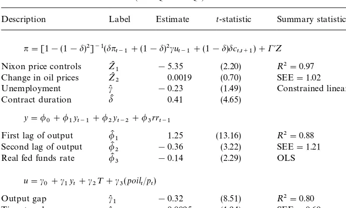
The estimates for three equations are presented in Table 1. For the price
Table 1
Estimates of basic contract model (1972Q1}1996Q4)!
Description Label Estimate t-statistic Summary statistics
n"[1!(1!d)2]~1(dn
t~1#(1!d)2cut~1#(1!d)dct,t`1)#C@Z (A)
Nixon price controls ZK1 !5.35 (2.20) R2"0.97 Change in oil prices ZK2 0.0019 (0.70) SEE"1.02
Unemployment c( !0.23 (1.49)
Contract duration dK 0.41 (4.65)
Constrained linear IV
1 !0.32 (8.51) RSEE"0.602"0.80
Time trend c(
2 0.0095 (1.94)
Relative price of oil c(
3 0.86 (5.56) 2SLS
!Data:*poilchange in oil prices is a four-quarter moving average of the price of oil imported into the U.S.;nis the quarterly change at annual rates of the chain-weight GDP price index;uis the demographically corrected unemployment rate, less the natural rate of unemployment from the FRB/US model database; c
t`1 is proxied by the median of the Michigan survey of expected
in#ation, 12 months ahead;yis the output gap for the U.S. from the FRB/US model database;rris the real interest rate de"ned as the quarterly average of the federal funds rate less a four-quarter moving average of the chain-weight GDP price index;poil/pis the price of imported oil relative the GDP price index; and Nixon price controls equals unity in 1971Q4 and!0.6 in 1972Q1. All regressions also included an unreported constant term. Constants were never statistically signi"cant. B}G(1) is the probability value of the Breusch}Godfrey test of"rst-order serial correlation.
Notes: Eq. (A) is estimated with instruments: constant, time trend, lagged unemployment gap, four lags of the change in imported oil prices; two lags of in#ation, lagged real interest rate, lagged Nixon wage-price control dummy, and the lagged relative price of imported oil. Standard errors for all three equations were corrected for autocorrelated residuals of unspeci"ed form using the Newey}West (1987) method.
the deviation of the demographically adjusted unemployment rate less the
NAIRU } were superior to those for output gaps. So the estimation was
conducted with that measure of economic slack, and the model was
supple-mented with a simple Okun's Law relationship linking the unemployment rate
to the output gap, as shown in the table as Eq. (C). We also embellished the basic
formulation with a small number of exogenous supply shock terms, speci"cally
7Chada et al. (1992)"nd stickiness of 0.55. See their Table 3, row 1. Laxton et al. (1999) and Fuhrer (1997)"nd stickiness of about 0.85.
8An able reference for state-space forms of linear rational expectations models and other issues in policy design is Holly and Hughes Hallett (1989).
and a constant term. These are traditional and uncontroversial inclusions. For example, Roberts (1996) has found oil prices to be important for explaining
in#ation in estimation using Michigan survey data.
The key parameters are the&contract duration'parameter,dK, and the excess
demand parameter, c(. When Eqs. (1) and (2) are solved, dK"0.41 implies
a reduced-form coe$cient on lagged in#ation of 0.63. To put the same
observa-tion di!erently: in#ation is 63% backward looking and 37% forward looking.
This level of in#ation stickiness is well within the range of estimates in the
literature from similar models; in#ation here is stickier, for example, than in
Chada et al. (1992) but less sticky than in Laxton et al. (1999) and Fuhrer (1997).7 With these estimates, our model is a generalization of the autoregressive
expec-tations Phillips curves exempli"ed by Gordon (1990) and Staiger et al. (1997)
which do not allow policy to a!ect expectations. Our model also generalizes on
theoretical Phillips curves such as those of King and Wolman (1999) and
Rotemberg and Woodford (1999). These speci"cations allow no stickiness in
in#ation whatsoever and, as Estrella and Fuhrer (1998) demonstrate, are
rejec-ted by the data. As for the output elasticity with respect to the real interest rate, c, the coe$cient bears the anticipated sign and is statistically signi"cant.
3. Methodology
3.1. Optimal and simple policy rules
It is useful to express the model in its"rst-order (state-space) form. To do this
we begin by partitioning the vector of state variables into predetermined
variables and&jumpers', and expressing the structural model as follows:8
K
core in#ation, our one non-predetermined variable. Constructing the
state-space representation for the model for a given policy rule is a matter of"nding
9This is because the optimal control rule cannot be expressed as a function of the nonpredeter-mined variables since these&jump'with the selection and operation of the rule. Rather, the rule must be chosen with regard to costate variables associated with the non-predetermined variables.When these costate variables are solved out for state variables, the resulting rule is a function of the entire history of predetermined state variables. In many cases, this history can be represented by an error-correction mechanism, as Levine (1991) shows, but not always. In any case, even when an error-correction mechanism exists, the basic point remains that the complexity of the rule is signi"cantly enhanced by the presence of forward-looking behavior.
Eq. (7) are recursive in the state variables so that manipulating the model is simple. This makes computing optimal rules a reasonably straightforward
exercise. However, two problems arise in the construction ofK.
The"rst of these problems is a technical one having to do with the fact that
K
1 is often singular. To solve this problem we exploit fast, modern algorithms
for solving singular systems developed by Anderson and Moore (1985) and advanced further by Anderson (1999). The second problem is more interesting
from an economic point of view and concerns "nding a speci"c rule with the
desired properties. This is an exercise in control theory. In the forward-looking context, however, the theory is a bit more complex than the standard textbook
treatments. The optimal control rule is no longer a function just of the"ve state
variables of the model as is the case with a backward-looking model. Rather, as Levine and Currie (1987) have shown, the optimal control rule is a function of
the entire history of the predetermined state variables.9Even for simple models
such as this one, the rule can rapidly become complex.
It may be unreasonable to expect agents to obtain the knowledge necessary to form a rational expectation of a rule that is optimal in this sense. Our
experi-ments have shown that agents have great di$culty learning the parameters of
rules with many conditioning variables. This is particularly so when some
variables, such as core in#ation,c, and price in#ationn, tend to move closely
together. In small samples, agents simply cannot distinguish between the two; unstable solutions can often arise. Rather than demonstrate this intuitively obvious result, in this paper, we consider instead restrictions on the globally optimal rule, or what we call simple optimal rules. Simple optimal rules are
those that minimize a loss function subject to the model of the economy}just as
regular optimal control problems do } plus a constraint on the number of
arguments in the reaction function.
For our purposes, we can state the monetary authority's problem as
argmin
subject to the state-space representation of the model as in Eq. (6), along with
the consistent expectations restrictions: m
10We also assume the existence of a commitment technology that permits the monetary authority to select and retain the rule that is optimal for given initial conditions, on average. Were we to assume that the monetary authority does not discount the future, we would not need a commitment technology. However, in order to conduct welfare comparisons along the transition path to di!erent rules, we need to discount the future. The strength of our assumption regarding commitment technology will be directly related to the rate of discounting. We use a low discount factor of 0.9875, or 5% per year on a compounded annual basis.
11We are taking a bit of license here, with our characterization of the Taylor rule, in that in#ation in the original speci"cation of the rule appears with a four-quarter moving average of in#ation and both in#ation and output appear contemporaneously. We take this simpli"cation to reduce the size of the state matrix for computational reasons.
arguments of the reaction function, (5): R
t"rrH#nt@t~1#bR[Rt~1! n
t~1]#bn[nt~1!nH]#byyt~1#uRt.10Loss functions of the form of Eq. (8)
are common in work with New Keynesian models (see, e.g., Taylor, 1979;
Williams, 1999). Moreover, Rotemberg and Woodford (1999, pp. 70}74) show
how such objectives can be justi"ed as close approximations to a social welfare
function in the context of an intertemporal optimizing model.
The solution to this problem, which is described in some detail in Appendix A,
is a vector of policy rule coe$cients, b"Mb
y,bn,bRN corresponding to the
vector of objective function weights,w"Mt
y,tn,t*RN.
Rules that solve the above problem will, by de"nition, be inferior to the
globally optimal rule that could have been derived using optimal control techniques, in the presence of full information. By the same reasoning, they will
be superior to even simpler rules such as the Taylor rule, with coe$cients
that are not chosen according to optimization criteria. In our formulation,
the Taylor rule is just our Eq. (5) with the added restrictions that b
R"0,
b
y"bn"0.5:11
R
t"rrH#nt@t~1#0.5[nt~1!nH]#0.5yt~1#uRt. (9) Eqs. (5) and (9) are the two policy rules that may be in force in our experiments.
The coe$cients in these rules are what agents are assumed to learn. The simple
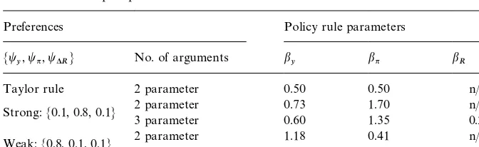
optimal rules derived from the above procedure are summarized in Table 2.
3.2. Learning
Our generic policy rule, Eq. (5), represents a single row of the matrix in Eq. (7), the values of which evolve over time according to recursive linear learning rules. Let us re-express Eq. (5), slightly more compactly as
R
t"bMtxt#u(Rt. (10)
Eq. (10) merely stacks the right-hand side arguments to the policy rule into
a vector,x
Table 2
Coe$cients of simple optimal rules!
Preferences Policy rule parameters
Mt
y,tn,t*RN No. of arguments by bn bR
Taylor rule 2 parameter 0.50 0.50 n/a
Strong:M0.1, 0.8, 0.1N 2 parameter3 parameter 0.730.60 1.701.35 n/a0.27
Weak:M0.8, 0.1, 0.1N 2 parameter3 parameter 1.181.55 0.410.53 !0.33n/a
!Notes: Rule parameters are the solutions to the problem of minimizing Eq. (8) subject to (6) and (5) under model consistent expectations, for the loss function weights shown in the"rst column of the table. The terms&strong'and&weak'refer to the strength of preferences for in#ation stabilization, relative to output stabilization.
coe$cients,bKt. Note that the caret overuRindicates that it, too, is a perceived
object. We discuss below how this works. Let the time series ofx
t beXt; that is,
X
t"Mxt~iDt0NWe assume that agents use either least squares or discounted least
squares to update their estimates ofbKt. Harvey (1993, pp. 98, 99) shows that the
recursive updating formula in Eq. (11) is equivalent to continuous repetition of an OLS regression with the addition of one observation:
bK
t"bKt~1#Pt~1xt(R!x@tbKt~1)f~1t , (11)
where P
t is the&precision matrix', Pt"(X@tXt)~1, and ft"1#x@tPt~1xt is a
standardization factor used to rescale prediction errors,u(
rs,t"Pt~1xt(R!x@tbKt~1), in accordance with changes in the precision over time. The precision matrix can be shown to evolve according to
P
t"jPt~1!Pt~1xtx@tPt~1f~1t . (12)
The parameter j is a &forgetting factor'. The special case j"1 discussed in
Harvey (1993) is standard recursive least squares (RLS). If we assume that agents have&less memory'we can downweight observations in the distant past relative
to the most recent observations by allowing 0(j(1. This is discounted
recursive least squares (DRLS).
The memory of the learning system has a convenient Bayesian interpretation in that had there never been a regime shift in the past, agents would optimally place equal weight on all historical observations as with RSL. Under such circumstances, the Kalman gain in Eq. (11) goes to zero asymptotically, and
bKPbM. However, if there has been a history of occasional regime shifts, or if
12Forgetting factors of 0.8 and below tended to produce instability in simulation. But discount factors this low represent half-lifes of memory of only about four quarters which we would regard as implausibly low.
shifts, the lower isj. Taking j(1 as an exogenously"xed parameter,bK will
have a tendency to#uctuate aroundbM, overreacting to surprises owing to the
maintained belief that a regime shift has some likelihood of occurring. That
agents overreact, in some sense, to&news'means agents with less memory will
tend to learn new rules more rapidly, but this rapid learning is not necessarily welfare improving.12
Whatever the precise form, using some form of learning here is a useful step forward since it models agents on the same plane as the econometrician, having to infer the law of motion of the economy from the surrounding environment, rather than knowing the law of motion a priori.
The policymaker's problem is to choose a policy rule of the form of Eq. (5), to
minimize the loss function, Eq. (8), subject to the model, Eq. (6). The problem of
learning adds the restriction that expectations are model consistent from the
point of view of private agents. This presents some challenging computational issues. Under model consistent expectations, solutions for endogenous variables depend on expected future values of other endogenous variables, which are
conditional on agents' (possibly incorrect) beliefs of monetary policy. Space
limitations prevent us from discussing the intricacies of the solution method here; they are described in some detail in the working paper version of this paper (Tetlow and von zur Muehlen, 1999).
4. Simulation results
One of our exercises is to consider the consequences of thecomplexityof rules
for welfare, given that agents must learn the rule in use. The error-correction representation of the optimal control rule contains seven arguments. In
prin-ciple, we could consider the di!erence in performance of this globally optimal
rule with that of a very simple rule. However as we have already noted, it is
di$cult for agents to learn rules with large sets of variables, in small samples
at least. Moreover it is di$cult to convey results over a large number of
parameters. To keep the problem manageable, we focus mostly on learning 3-parameter optimal rules, beginning from 2-parameter rules.
We also examine the costs of transitions from an ad hoc (sub-optimal) rule}
our version of the Taylor rule}to an optimal 3-parameter rule, as well as from
13Our quantitative work has shown the Taylor rule both as it is written in Taylor (1993), and as we have written it here, works satisfactorily in a wide range of models.
re#ects the familiarity of the Taylor rule to a large cross-section of economists
involved in monetary policy debates. In addition, as Taylor (1993) argues, the Taylor rule approximates Fed behavior quite well over the 1980s.13
For our 3-parameter rules, we focus on the simple optimal rules described
above, for a variety of preferences, of which we concentrate on two di!erent
sets. All of the rules we examine can be considered in#ation-targeting rules
in that each places su$cient emphasis on a "xed target rate of in#ation to
ensure that this rate will be achieved, on average, over time. The two rules we
concentrate on di!er with regard to how aggressively they seek this goal, relative
to other objectives. An authority that places a large weight on in#ation
stabiliz-ation}a weight of 0.8 in our formulation}is said to have strong preferences
for in#ation targeting. For conciseness, in most instances we shall call
this authority &strong'. Strong in#ation-targeting authorities are weak
output targeting authorities since they place a weight of just 0.1 on output
stabilization. Symmetrically, an authority that places a weight of 0.1 on in#ation
stabilization and a weight of 0.8 on output stabilization shall be referred to as
having relatively weak tastes for in#ation targeting and shall be referred to as
&weak'.
With all sets of preferences, we place a weight of 0.1 on restricting the variability of the nominal federal funds rate. A monetary authority may be concerned with the variability of its instrument for any of a number of reasons. First, and most obviously, it may inherently prefer less variability as a matter of taste, either in its own right, or as a device to avoid criticism of excessive activism. Second, constraining the volatility of the federal funds rate might be
a hedge against model misspeci"cation. Finally, as Goodfriend (1991) argues,
interest-rate smoothing may expedite expectations formation in
forward-look-ing economies. These taste parameters and the rule coe$cients they imply are
summarized in Table 2.
Finally, we conduct many of these experiments using three di!erent degrees of
memory. The"rst is full recursive least squares (j"1), which we shall refer to as
&full memory'. The other two cases are discounted recursive least squares
(DRLS), one with somewhat limited memory (j"0.95), which we will call&long
memory'and another with &short memory': (j"0.85). The long memory case
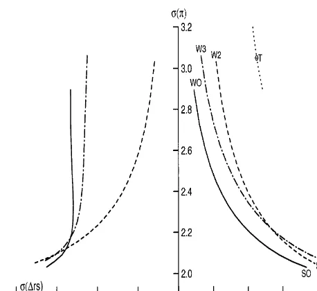
Fig. 1. Selected optimal policy frontiers.
14The convexity to the origin of the frontier arises because shocks to the Phillips curve change in#ation which can only be o!set by the authority inducing movements in output. If movements in in#ation came about solely because of shocks to demand, no policy dilemma would arise and no curve as such would exist.
4.1. The rules in the steady state
Let us build up some intuition for what follows with an examination of the optimal policy rules in steady state. The parameters of the strong and weak
in#ation-targeting monetary authority's rules are summarized in Table 2, along
with the parameters of our version of the Taylor rule. The mapping of penalties,
measured by thet
i,i"My,n,*RN, and therelativemagnitudes of the policy rule
parameters,b
j,j"My,n,RN, is as one would expect: a larger coe$cient on, say,
t
nThe performance of the complete set of rules with, results in a larger coe$cient onbn relative tobyt.
*R"0.1 and preferences
for the range of weights on t
y, tn bounded between 0.1 and 0.8, with
t
y#tn"1, are summarized in Fig. 1. The"gure shows the trade-o!s between
the standard deviations of in#ation and output in the steady state in the
right-hand panel, and between in#ation variability and the variability of the
change in the federal funds rate in the left-hand panel.14
First make note of the lower three curves in the right-hand panel. The solid
15This is not shown in the left-hand panel of the"gure in order to maintain visual clarity.
16For example, the same general"nding that the Taylor rule is&weak'in the sense described in the text and averse to interest-rate variability arises with the FRB/US model of the U.S. economy maintained by the Federal Reserve Board, albeit somewhat less dramatically so. This"nding may re#ect either the policy preferences in play over the period to which the Taylor rule was loosely
"tted, or it may re#ect the relatively placid nature of the shocks over the period.
variables appear. The dot-dashed frontier immediately to the north east of the globally optimal frontier is associated with the optimal 3-parameter rule, while the dashed frontier is the optimal 2-parameter frontier. The strong and weak rules are, respectively, at the bottom and top of each of the curves, with SO
representing the strong rule generated from optimal control, S2 the optimal
2-parameterstrong rule, and so on.
The "rst and most obvious thing to note about these frontiers is that the globally optimal rule is closest to the origin, meaning it produces superior
performance to all other rules, measured in terms of output and in#ation
variability. A more interesting result is that the 3-parameter and 2-parameter
frontiers cross. This crossing re#ects the fact that movement along the
2-parameter rule frontier towards more strong preferences involves a much larger
sacri"ce in terms of higher interest-rate variability than for the 3-parameter rule.
Evidently, in#ation control and interest-rate control are strong substitutes, at
the margin, for the strong policymaker. That this is so in the neighborhood of the strong rules, and not so in the vicinity of the weak rules, is an observation we shall return to below when we discuss transitions from 2- to 3-parameter rules in Section 4.3.
The point marked with a &T' in the right-hand panel is the Taylor point
representing the performance of the Taylor rule in this model. This rule performs substantially worse than any optimal 2-parameter rule in terms of output and
in#ation variability, but at 3.0 percentage points, produces a substantially lower
standard deviation of the change in the federal funds rate.15It follows that there
is a set of preferences for which the Taylor rule is optimal in this model. Some
computation reveals that a coe$cient of about 0.5 on the change in the federal
funds rate produces an optimal frontier that slices through the Taylor point as shown. Thus, a policy maker that uses the Taylor rule is very reluctant to allow
#uctuations in the policy instrument.
The steepness of the frontier at the Taylor point also shows that this version of the Taylor rule is very weak in that a monetary authority that would choose this point is apparently willing, at the margin, to accept a very large increase in
in#ation variability to reduce output variability only slightly. While this result is
17This experiment is broadly similar to Fuhrer and Hooker (1993), who also consider learning policy parameters. However, they do not consider optimal rules and do not examine the welfare implications of the choice of rules.
18In order to ensure the lags and the precision matrix were properly initiated according to pre-experiment conditions, 200 periods were simulated using the initial rule before shifting to the new rule. For each experiment, 300 periods were simulated and each experiment comprised 3000 draws so that altogether each of the major experiments reported in this paper involved computing 900,000 points. On a single processor of an UltraSparc 4 296 megahertz UNIX machine, each experiment took a bit over 3 hours to compute.
4.2. Changes in preferences
Having examined the steady-state performance of our rules, let us now consider transitions from one rule to another. In order to keep things simple, we shall focus initially on changes in policy preferences using 2-parameter rules. In particular, the thought experiment we have in mind is of a newly installed
policymaker, replacing an incumbent of quite di!erent preferences. The new
authority has to decide whether to switch to a new rule that is consistent with its
preferences. The new rule will produce better steady-state performance}from
the point of view of the new authority}but presumably only after bearing some
transitional costs as agents learn of the new rule. It is conceivable that the transitional costs could be so high that the new authority would prefer to continue to govern policy with the old rule, even though it is inconsistent with its
steady-state preferences.17
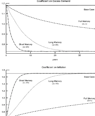
Fig. 2 shows the evolution over time of the parameter estimates for the
transition from a regime of weak preferences for in#ation control, to a strong
one, using the 2-parameter optimal rules. (Henceforth, we shall drop the label
&optimal'except where this would cause confusion.) The upper panel shows the
perceived coe$cient on excess demand and the lower panel shows the coe$cient
on in#ation. In each panel, we also show a base case }the solid line}where
agents believe the initial regime will continue, and they are correct in this expectation. For all the other cases, their prior expectations turn out to be
incorrect. The dashed line is the &full memory' case. The dotted line is &long
memory'learning case (that is, discounted recursive least-squares learning with
j"0.95). The dot-dashed line is&short memory'case (DRLS withj"0.85). The lines in each case are the average values over 4000 draws. Each simulation lasts
200 periods.18
Let us concentrate, for the moment, on the upper panel of Fig. 2. The"rst
thing to note from the"gure is the obvious point that agents do not get fooled in
Fig. 2. Perceived policy rule parameters. Learning a shift from&weak'to&strong'in#ation-control preferences (average of 4000 draws).
More important than this, however, is the observation that regardless of which of the three learning devices that is used, it takes a remarkably long time for agents to come to grips with the change in parameters. In particular, with full
memory, agents have not learned the true rule coe$cients even after the"fty
years covered in the experiment. Even under rapid discounting of j"0.85 }
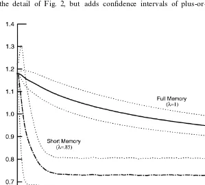
Fig. 3. Perceived coe$cient on excess demand. Learning a shift from&weak'to&strong'in# ation-control preferences (with$1 standard error bands).
more than ten years before agents reach the new parameter values. This"nding,
which is consistent with earlier results, such as those of Fuhrer and Hooker (1993), stems from two aspects of the learning rules. First, the speed of updating is a function of the signal-to-noise ratio in the learning mechanism. Because a considerable portion of economic variability historically has come from random sources, agents rationally infer the largest portion of surprises to the observed federal funds rate settings as being noise. Accordingly, to a large extent, they ignore the shock. Second, these results show how linear learning rules tolerate systematic errors; the forecast errors that agents make get increas-ingly smaller, but are nonetheless of the same sign for extended periods of time. A non-linear rule might react not just to the size of surprises, but also a string of errors of one sign.
The bottom panel of Fig. 2 shows the evolution of the perceived coe$cient on
in#ation. A"gure showing the learning rates when a strong in#ation-targeting
regime is succeeded by a weak one is similar to Fig. 2.
We can derive a third observation, this time from Fig. 3, which repeats some
19Loss"gures shown are the average over the 4000 draws conducted. A quarterly discount factor of 0.9875, is applied in computing the losses. This is a modest discount factor, in line with what might be used in"nancial markets. The substantive facts presented in this paper were invariant to the choice of discount factors, at least within a range we would consider to be reasonable. Political economy arguments might yield positive arguments for a substantially lower discount factor, but this is not the subject of this paper.
standard error around the coe$cient means for the full-memory and
short-memory cases. The bands show us that as agents increasingly discount the past
in forming their expectations, the coe$cient estimates become less and less
precise, particularly in the early going of the learning exercise. Also, as one might expect, there is considerably more variability around the steady-state estimates of the policy parameters under the short memory case than there is under the full memory case. Our experiment is a once-and-for-all regime shift; private agents, however, perceive shifts as regular occurrences. They keep a watchful eye for evidence of additional shifts and consequently overreact to purely random
errors. The"gure does not show the full memory case after it converges on the
true policy parameters but it is evident from the"gure, and demonstrable from
the data, that the variability ofbK is lower in the steady state under full memory
than it is under short memory.
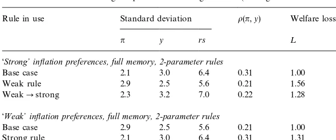
Table 3 summarizes the welfare implications of this experiment. The table is
divided into two panels. The top panel shows the decision a strong in#
ation-targeting policy maker would have to make after succeeding a policy maker with
weak preferences for in#ation targeting. The row in this panel labeled&base case'
shows the performance that the economy would enjoy had the strong policy rule
been in e!ect at the outset. This can be thought of as the &after picture'. The
second row, labeled&weak', shows the performance of the economy under the
weak rule; that is, the rule that was in place when the strong policymaker took
over. This is the&before picture'. Finally, the third row shows the transition from
the weak rule to the strong one. The key column of the panel is the far right-hand column showing welfare loss. This is the average discounted loss
under the policies,measured from the perspective of the incoming strong
policy-maker.19In terms of the raw numbers, the performance of the economy under,
say, the weak rule as shown in the second row, will not be any di!erent than it
was under the weak regime, but the loss ascribed to this performance can di!er
markedly depending on the perspective of the policymaker.
To aid comparison, we have normalized the loss"gures for the base case to
unity. By comparing the third row of the upper panel with the"rst row, we can
see the loss associated with having to learn the new rule. By comparing the third row with the second row, we can see whether the transition costs of learning the new rule are so high as to induce the new policymaker to stay with the old rule.
Table 3
Simulation results from change-in-preference learning exercises (Average across 4000 draws)!
Rule in use Standard deviation o(n,y) Welfare loss
n y rs ¸
&Strong+inyation preferences, full memory, 2-parameter rules
Base case 2.1 3.0 6.4 0.31 1.00
Weak rule 2.9 2.5 5.6 0.21 1.56
WeakPstrong 2.3 3.2 7.0 0.22 1.28
&Weak+inyation preferences, full memory, 2-parameter rules
Base case 2.9 2.5 5.6 0.21 1.00
Strong rule 2.1 3.0 6.4 0.31 1.31
StrongPweak 2.4 2.5 5.1 0.33 0.93
!Notes: The"rst row of each panel contains the&base case'results de"ned as those corresponding to the optimal 2-parameter rule for the policy preferences noted; the row immediately below each base case is the performance of, and loss to, staying with the 2-parameter policy rule inherited from the previous regime. The third row shows the performance and cost of changing from the inherited regime to the (new) optimal 2-parameter rule. Qualitatively similar results were derived using 3-parameter rules and using discounted recursive least-squares learning.
correlation of output and in#ation in the simulated data. Comparing this across
experiments gives an indication of the extent to which the monetary authority is
using the Phillips curve trade-o!to achieve its objectives. The"rst two entries in
this column of the table show that a strong in#ation targeter induces a stronger
correlation than does a weak in#ation targeter, re#ecting the need for in#ation
control to operate through manipulating current and expected future levels of excess demand.
The bottom panel of the table is analogous to the top panel, except that the
transition is from a former strong in#ation-targeting regime to a new weak
regime.
Turning to the results themselves, in the case of the incoming strong policy-maker, the process of learning is costly relative to the base case; not being able to simply announce a new policy regime and have private agents believe it, implies substantial costs. However, the comparison of rows two and three shows that the incoming strong policymaker would be willing to bear the transition costs of switching rather than stick with the incumbent rule.
A more intriguing case is the transition from a strong policy regime to a weak one, shown in the lower panel. The third row of the lower panel shows that the
weak policymaker actually bene"ts from the prior belief of private agents that
by de"nition, the base case should yield the best result possible in the circum-stances. The reason why this intuition does not hold becomes clear once one recognizes that learning is breaking, in some sense, the model-consistency condition in the model. Notice that lower loss in the transition case comes from
reduced in#ation and federal funds rate volatility. The volatility of in#ation is, to
a large extent, determined by the expected future path of the model's jump
variable, core in#ation, c
t`1@t. However, future core in#ation is being pinned
down by the expectation that monetary policy in the future will restrain future
in#ation with the strong rule. This expectation turns out to be erroneous, of
course. From the policymaker's point of view, expectations are not model
consistent, even though they are from the point of the view of private agents. Thus, to the extent that learning is slow, the weak policymaker can indulge his
inclination to manage output without bearing the costs of incipient in#ation
pressures, and with reduced interest rate variability as well.
No similar bene"t is shown for the transition from weak to strong preferences
shown in the upper panel of the table. Two reasons account for this asymmetry.
The "rst of these relates to the fact that the monetary authority controls
in#ation primarily through its management of aggregate demand. To a
substan-tial degree, the belief by private agents that the authority will manage output
tightly is only bene"cial to the strong authority to the extent that in#ation
#uctuations originate from demand shocks. A large portion of in#ation
variabil-ity in the U.S. economy comes from shocks to the Phillips curve}that is, from
so-called supply shocks. The larger the proportion of shocks to in#ation
origin-ating from supply-side sources, the more con#icts arise in the management of
demand and the control of in#ation. This e!ect is not at work when moving
from the strong to weak preferences, because demand management comes at an
earlier stage in the monetary transmission mechanism than does in#ation
control. The second reason is that there is no jump variable in output in this model. This leaves expected future demand less important for current demand
management than is the case for in#ation. It follows that a strong monetary
authority wants to credibly announce regime changes when taking over from a weak incumbent, while a newly installed weak policymaker wants to conceal
his true preferences and possibly forestall private agents'learning as much as
possible.
The observation that weak policymakers gain from being perceived as strong,
because doing so decouples in#ation expectations from policy actions for a time,
echoes the theoretical literature on policy games. In Vickers (1986, pp. 451, 452),
for example,&wet' policymakers will be better o!by passing themselves o! as
&dry'policymakers in the presence of incomplete information than they would be
under full information. In contrast,&dry'policymakers will usually be better o!
under full information.
20The base-case loss is independent of the&memory'in the learning process.
21This and all subsequent equivalent variation calculations are measured relative to the base-case rule.
22Tetlow and von zur Muehlen (1996) report a similar"nding with another small model as does Williams (1999) with the FRB/US model which has some 300 equations.
settings as a signal, in some sense, that the policy rule had changed. Results not shown here demonstrate that learning can be accelerated, but at the cost of higher losses than under base-case learning. The details of these experiments can be found in the working paper version of this article: Tetlow and von zur Muehlen (1999).
4.3. Learning to be optimal
Now let us consider agents who begin with the 2-parameter rule who must then learn that the Fed has shifted to one of our simple optimal rules laid out in
Table 2. We consider"rst the results for strong in#ation-targeting preferences,
summarized in Table 4. For ease of comparison the loss for the base-case row,
which is the optimal 3-parameter rule in this case, normalized to unity.20The
"rst panel of the table shows the performance of the economy under the three alternative steady states; it corresponds to Fig. 1. Having already examined Fig.
1, it is not surprising that the Taylor rule's performance features substantially
higher in#ation variability than the strong base-case rule, but lower variability
in output and especially the federal funds rate. The Taylor rule's performance
also shows substantially more persistence in in#ation and interest rates (not
shown) and a higher correlation of output and in#ation, indicating that policy is
working more through the traditional Keynesian channel, rather than through expectations, than in the base case. From the point of view of a strong pol-icymaker, the Taylor rule is seen as a poor performer. Measured in terms of discounted loss, the Taylor rule is 56% worse than the 3-parameter rule. Putting
the same performance a di!erent way, the strong policymaker would just as
soon accept an autonomous increase in the variance of in#ation of
three-quarters of a percentage point or a whopping 3.1% in output variability as be
forced to use the Taylor rule.21
The second row of the table shows the performance of the 2-parameter rule. Relative to the base case, there is only a 2% loss from using the 2-parameter rule.
The strong authority would be willing to sacri"ce output variability of 0.2
percent in order to avoid using this rule. While this is not trivial, it is also not
large. Thus, a signi"cant"nding in this paper is that the gains in steady state
from using even slightly more complex rules than a 2-parameter rule is small}at
least for strong preferences }provided that the simpler rule's parameters are
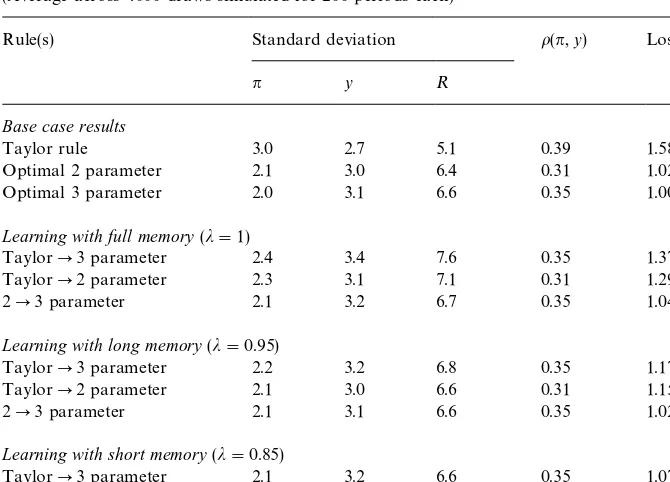
Table 4
Learning under strong preferences for in#ation targeting (Average across 4000 draws simulated for 200 periods each)!
Rule(s) Standard deviation o(n,y) Loss¸
n y R
Base case results
Taylor rule 3.0 2.7 5.1 0.39 1.58
Optimal 2 parameter 2.1 3.0 6.4 0.31 1.02
Optimal 3 parameter 2.0 3.1 6.6 0.35 1.00
Learning with full memory(j"1)
TaylorP3 parameter 2.4 3.4 7.6 0.35 1.37
TaylorP2 parameter 2.3 3.1 7.1 0.31 1.29
2P3 parameter 2.1 3.2 6.7 0.35 1.04
Learning with long memory(j"0.95)
TaylorP3 parameter 2.2 3.2 6.8 0.35 1.17
TaylorP2 parameter 2.1 3.0 6.6 0.31 1.15
2P3 parameter 2.1 3.1 6.6 0.35 1.02
Learning with short memory(j"0.85)
TaylorP3 parameter 2.1 3.2 6.6 0.35 1.07
TaylorP2 parameter 2.1 3.0 6.4 0.31 1.07
2P3 parameter 2.1 3.1 6.6 0.35 1.01
!Notes: The syntax&nPm'refers to the results from learning the transition from then-parameter simple optimal rule to them-parameter simple optimal rule. Losses are computed as discounted loss with a discount factor equal to 0.9875.
rule, but markedly di!erent coe$cients, as Table 2 shows. Obviously, there are
large gains to be had from picking rule parameters judiciously.
Now let us consider the decision by a strong policymaker, of whether to shift from a Taylor rule to the 2-parameter rule as well as to the 3-parameter rule. To
separate the e!ects of optimality from complexity, we also consider moving from
the 2-parameter rule to the 3-parameter rule. We conduct these exercises with
full memory (j"1 in the second panel of Table 4), long memory (third panel),
and short memory (bottom panel). The"rst thing to note about the results is
that when agents have to learn about rule changes, short memory is a good thing. The loss for the short-memory cases are less than for the corresponding long-memory cases, which in turn are lower than the full-memory cases,
regard-less of which learning exercise one considers. Since the variability of bK varies
inversely withj, this result is not trivial. It would stand to reason that greater
23The weak policymaker would be willing to permit the variance of output to rise by 0.3 in order to avoid using the Taylor rule. Recall from earlier that the strong policymaker would tolerate a 0.75 increase in in#ation to avoid the same fate. (In#ation carries the same 0.8 weight in the strong policymaker's loss function as output does in the weak's loss function.).
24This can be seen in Fig. 1 by comparing the very steep slopes of the trade-o!s between the variability in the change in the federal funds rate and the variance of in#ation in the neighborhood of the weak rules, with the much#atter slopes of the same curves in the neighborhood of the strong rules.
with higher losses in the steady state. These higher steady-state losses could
o!set the lower transitional losses as the steady state is approached. In fact, the
di!erence in the steady-state loss between the short-memory case and the
full-memory case is negligible, meaning that, for these cases at least, only the transitional losses matter.
A second observation from Table 4 is that regardless of how slow the learning is, the strong policymaker is always willing to bear the transitional costs of moving from the Taylor rule to either the 3-parameter or 3-parameter optimal
rules (compare the loss column of the"rst row with any row in the bottom three
panels). More intriguingly, however, in some cases, the strong authority is better
o!moving to the 2-parameter rule than moving directly to the 3-parameter rule.
This is so even though the cost of moving from the 2-parameter rule to the
3-parameter rule is generally small. The reason is, of course, that the bene"ts are
often smaller still.
Now let us examine the same experiment for weak preferences for in#ation
control, shown in Table 5. The mass of numbers in the table yield essentially one point: regardless of whether one begins from the Taylor rule or from the 2-parameter (weak) rule, and regardless of the memory in the learning
mecha-nism, there is very little di!erence in the loss. Simply put, neither the speed of
learning, nor the complexity of the rule, makes a substantial di!erence in terms
of welfare. To see why this is so, "rst consider the welfare loss to a weak
policymaker from pursuing the Taylor rule. The loss is certainly
consequen-tial,23 but given the vast distance the Taylor rule coe$cients are from the
optimal 2-parameter rule coe$cients, the di!erence in performance seems small.
Simply put, the loss function for the weak policymaker is very#at, or, to put the
same observation another way, relatively crude control methods yield broadly similar economic performance, for weak preferences.
This#atness of the loss function arises because managing output#uctuations
to the near-exclusion of other objectives is a relatively easy task. This is so for
three reasons. First, as we noted above with regard to Fig. 1, in#ation control
and interest-rate smoothing tend to be substitutes. The con#ict raised by this
substitutability is a slight one for the weak policymaker who is largely
Table 5
Learning under weak preferences for in#ation targeting (Average across 4000 draws simulated for 200 periods each)!
Rule(s) Standard deviation o(n,y) Loss¸
n y R
Base case results
Taylor rule 3.0 2.7 5.1 0.39 1.12
Optimal 2 parameter 2.9 2.5 5.6 0.21 1.02
Optimal 3 parameter 3.0 2.4 5.6 0.20 1.00
Learning with full memory(j"1)
TaylorP3 parameter 2.8 2.4 5.6 0.27 0.99
TaylorP2 parameter 2.8 2.5 5.6 0.29 1.01
2P3 parameter 2.9 2.4 5.5 0.21 0.99
Learning with long memory(j"0.95)
TaylorP3 parameter 2.9 2.4 5.6 0.22 1.00
TaylorP2 parameter 2.9 2.5 5.6 0.23 1.01
2P3 parameter 2.9 2.4 5.6 0.20 1.00
Learning with short memory(j"0.85)
TaylorP3 parameter 2.9 2.4 5.6 0.20 1.00
TaylorP2 parameter 2.9 2.5 5.6 0.21 1.02
2P3 parameter 3.0 2.4 5.6 0.20 1.00
!Notes: The syntax&nPm'refers to the results from learning the transition from then-parameter simple optimal rule to them-parameter simple optimal rule. Losses are computed as discounted loss with a discount factor equal to 0.9875.
depend in an important way on forward expectations. This means that agents'
prior expectations of what rule is in place is of lesser importance for the weak authority. Third, output appears earlier in the monetary policy transmission mechanism that links funds rate setting, to output determination and then
in#ation.
Taken together, the results shown in Tables 4 and 5 send a cautionary message about how a monetary authority should select among candidate rules. For some preferences, any vaguely sensible rule will perform reasonably well.
However, the more the authority is concerned with in#ation control, the more
5. Concluding remarks
This paper has examined the implications for the design of monetary policy rules of the complexity of rules and the interaction of complexity and preferences with the
process of learning by private agents of the in#ation-targeting rule that is in place.
In particular, we took a small New Keynesian macroeconometric model and computed optimal simple rules for two sets of preferences: strong preferences for
in#ation control, where a substantial penalty is attached to in#ation variability
and only a small weight on output or instrument variability; and weak
prefer-ences for in#ation control, where the same substantial weight is placed on
output variability. Then we compared the stochastic performance of these policies that would have been optimal within a single regime to two types of
transition experiments. The"rst was the transition to more complex rules from
simpler rules, within a single regime. The second was the transition between regimes for a simple optimal rule of given complexity.
Our four basic "ndings are: (1) learning should be expected to be a slow
process. Even when agents&forget' the past with extraordinary haste, it takes
more than 10 years for agents to learn the correct parameters of a new rule. (2) The costs of these perceptual errors can vary widely, depending on the rule that is initially in force, and on the preferences of the monetary authority. In
particular, a strong in#ation-targeting monetary authority tends to"nd high
costs associated with the need for agents to learn a new (strong) rule that has been put in place. It follows that such a policymaker should be willing to take steps to identify his policy preferences to private agents. Paradoxically, a weak
policymaker will sometimes bene"t from being misperceived, posting a better
economic performance than would have been the case if the optimal rule had been in place all along. This sharp contrast in results has to do with the
multiplicity of sources of shocks to in#ation, the nature of in#ation in this model
being a forward-looking variable, and the fact that in#ation appears later in the
chain of the monetary policy transmission mechanism than does output. (3) The performance, in steady state, of optimal two-parameter policy rules is not much worse than the performance of optimal three-parameter policy rules, at least for this model. Largely for this reason, some policymakers that would like to move
from a suboptimal rule would be better o!moving to the optimal 2-parameter
rule, and forsaking the 3-parameter rule, than bearing the incremental costs of private agents having to learn the more complicated rule. (4) Faster learning is
not necessarily better. When the monetary authority takes steps to &actively
teach'private agents that the rule has changed, agents' expectations converge
more rapidly on the new and true parameters, but economic performance does not necessarily improve. This is because the policymaker himself must add instrument variability to the system in order to hasten the learning, and because
initial bene"ts of more rapid learning are&given back'when learning slows down
25See also Anderson (1999) for an updated derivation and description of the methodology. Appendix A
A.1. State-space representation of the model
In the main body of this paper, the following variable de"nitions are used:y
tis
log output gap,n
t is goods in#ation,Rt is an interest rate}in the present case,
the overnight borrowing rate under the control of the monetary authority, and
c
t is core or contract in#ation. The model is
y
2(0,/3(0, and Etis the expectations operator, given information in
period,t. All variables are measured as deviations from equilibrium, implying
that their steady states are zero. The authority commits to a policy rule,
R
t"nt#ut
,n
t!Fxt, (A.4)
whereu
tis the control variable,Fis a vector of constants to be determined, and
x
variables in the system, with z
0 given, and ct is the forward-looking jump
variable. We make the additional (rational expectations) assumption that E
tct`1
is consistent with the mathematical expectation ofc
t`1obtained by solving the
model using AIM, Anderson and Moore's (1985) generalized saddlepath
proced-ure available in MATLAB, GAUSS, and MATHEMATICA.25Accordingly, we
drop the E
t notation. In matrix form, the"rst-order autoregressive form of the
equations in (A.1)}(A.4) is,
C1x
26The AIM algorithm involves a number of pre-processing steps enabling it to solve for the state-space representations of very large linear dynamic rational expectations models whenever a model can be written as
h coe$cients before control;X
tis information int,qis the maximum lag (in our case 1), andhis the maximum lead (in our case 1). Having eliminated any singularities, AIM creates the transition matrix,C. Since inessential lags associated with nonsingularities have been eliminated, C
1 will
necessarily have smaller dimension than the singular left-hand matrix one normally builds for the state-space representation.
Premultiplying (A.5) byC~11 , yields the state transition equations,26
In the above representation, the state vector,x
t`1, evolves from its preceding
value intvia the transition matrix,C, modi"ed by the e!ect of the control,u
t,
and the unforeseen demand and supply shocks,g
t.
The policy authority targets in#ation, output, and changes in the short-term
interest rate. Accordingly, de"ne the vector,s
t"[Rt!Rt~1,yt,nt]@. Given the
The central bank seeks to minimize the expected present value of a weighted
sum of squared deviations of in#ation, output, and changes in the interest rate
from their respective (zero) targets. De"ning the diagonal 3]3 performance
metric,W
the expected loss to be minimized is
E=
where E is the expectations operator, as before, 0(o41 is the discount factor,
andR
s is the unconditional covariance matrix ofs, so that, asymptotically, the
authority is seeking to minimize a weighted sum of the unconditional variances of the three target variables.
In light of (A.8), the expected loss can be re-expressed as a function of the
Standard optimal control packages assume no discounting, o"1, and no
crossproducts,;"0. However, a simple transformation of the variables allows
us to translate the problem with crossproducts and discounting into a
conven-tional optimal control problem. To this end, de"ne
u(
In optimal control, we seek a vector,FM, satisfying
u(
t"!FMx(t, (A.13)
that minimizes the asymptotic expected loss (A.11) subject to (A.12). Substituting
(A.13) foru(
t in (A.11) and (A.12), E=0 is, equivalently,
E=
0"12tr[(WM #FM@NFM)Rx]#trMS[Rg!Rx#(CM!BMFM)Rx(CM!BMFM )@]N
27To show that this is so, letA"CM!BMFM, so that (A.12) becomes Thus, askbecomes large, the covariance ofx(
tis the covariance ofxt:
28Here we have exploited the facts that
L
x is the asymptotic covariance ofx,27
R
x"Rg#(CM!BMFM )Rx(CM!BMFM )@, (A.15)
andSis the 5]5 matrix of Lagrangian variables associated with the constraint
(A.15). Di!erentiating (A.14) with respect toFM andR
y, we determine the two
equations familiar from the control literature,28
FM"[N#BM@SBM]~1BM@SCM,
S"WM #(CM!BMFM )@S(CM!BMFM )#FM@NFM.
Finally, a feedback law for the orginal state variables, x
t, is retrieved by
observing that
u
t"!(FM#N~1;@)xt,!Fxt.
Formulation of an operational feedback rule is complicated by the fact that the
optimal control rule, (A.13) as solved, contains the expectational variable, c
t,
which itself, jumps with the selection of the rule. Based on a solution due to
Backus and Dri$ll (1986), one can express the optimal policy as a function of
solely the predetermined variables,z, by writing it"rst as a function of those
predetermined variables and the costate variables,p, associated with the
29Levine (1991) has pointed out that (17) is equivalent to an error-correction rule.
30(G
2¹~122)~1is a pseudo-inverse if the number of jumpers,m, is not equal to the number of
instruments,k, in the model, as is typically the case in macroeconomic models. A pseudo-inverse of a non-square matrix requires a singular-value decomposition of the matrix to be inverted and can be obtained, for example, with the MATLAB functionpinv.m.
where
21 andS22 are appropriately dimensioned partitioned submatrices ofS.
The indices,&1'and&2'correspond to the predetermined and non-predetermined
variables, respectively. Let¹"H(A!BF)H~1. Then the transition equation
forzandqis
Accordingly,qcan be expressed as a di!erence equation driven by the
predeter-mined variables,z
t,
p
t`1"¹22pt#¹21zt.
Given the policy rule (A.16), this can be written
p
t`1"¹21zt~q#¹22G~12 (ut!G1zt),
so that, solving foru
t and substituting forpt by lagging the preceding equation
once, we obtain
corresponding to the dimension ofz
t.29In the model of this paper, there is only
one non-predetermined variable and one control variable, soG
2¹~122 is a
scal-ar.30Eq. (A.17) shows that in a forward looking model, optimal policy in each
Since some lags ofR,n, andyappear more than once, we simplify (A.17) to obtain the seven-parameter optimal rule referred to in the text,
R
The&simple'policy rules considered in this paper are versions of (A.18),
u
t"KI wt,KI Jxt,
whereJis a 7]6 matrix that mapsx
t intowt, andKI has the same dimension as
K in (A.18) but may contain elements that are restricted to zero. De"ne the
transfer function,G(¸), mapping the disturbances,g
t, onto the output vector,st:
G(¸)"(M#M
uKI J)[I!(A#BKI J)¸]~1, where ¸ is the lag operator:
¸x
t"xt~1. Then, given a selection of k elements in KI that are allowed to
change, an optimalk-parameter rule is determined by constrained optimization
such thatKI satis"es
The minimum is determined iteratively, where, for this application, we used
MATLAB's constrained optimization function, constr.m, where, with each
ith trial KI i, the model is solved backward, using AIM, until a minimum is