*Corresponding author. Tel.: #33-556842407; fax: # 33-556846644.
E-mail address:[email protected] (Y. Ducq).
Coherence analysis methods for production systems by
performance aggregation
Yves Ducq*, Bruno Vallespir, Guy Doumeingts
Laboratoire d'Automatique et de Productique, GRAI Group, University Bordeaux 1, 351 Cours de la Libe&ration, 33405 Talence Cedex, France Received 2 April 1998; accepted 2 May 2000
Abstract
This paper aims at describing methods for the coherence analysis in production systems. This coherence between the various objectives of the decision system is analysed in order to ensure that the achievement of local performances allows the achievement of the global ones, assigned to the whole enterprise. The coherence analysis methods are usable for quantitative objectives, whatever the kinds of performance which is concerned (cost, quality, lead time,#exibility, etc.). The coherence analysis is based on the aggregation and comparison of expected performances (objectives) between the various decision levels. Various methods are developed in the frame of the concepts of the GRAI Model. ( 2001 Elsevier Science B.V. All rights reserved.
Keywords: Performance; GRAI Model; Coherence; Objectives; Aggregation
1. Introduction
The improvement of Enterprise Performance in order to get more bene"ts is a continuous expecta-tion of the enterprise Sta!Management.
Nevertheless, even if these objectives are always the same for more than 20 years, the means to achieve them have considerably evolved, due to the enterprise environment and competition on the one side and the evolution of production and produc-tion management techniques on the other. One of the main changes is, for the decision makers, to control their production system more and more precisely in order to improve continuously its
per-formances, mainly in terms of cost, lead time and product quality, and also in terms of reactivity and #exibility [1}5].
This performance, which was yesterday mono-criterion, mainly based on cost, is today multi-criteria [6,7].
In order to perform this accurate control, the decision makers must have a coherent objective system. It means that each decisional level must contribute to the achievement of global perfor-mance of the enterprise de"ned by the top manage-ment.
The objective of the research works presented in this paper is to contribute to a method, based on the GRAI Model [18], which allows to analyse and to correct the coherence of an objective system in order to ensure that the local (i.e. operational) objectives contribute to the achievement of global (i.e. strategic) objectives, it means that the local
performance achievement contributes to the achievement of global performance.
Thus, after the slight presentation of the GRAI Model concepts, the de"nition of the concept of objective will be given. Then, a typology is present-ed for the decomposition of &father' objective in &son' objectives. In a third time, the various methods to analyse and to correct the coherence will be presented, each one being adapted to each kind of decomposition.
2. State of the art of coherence analysis methods
There does not exist much work concerning coherence analysis methods in the domain of pro-duction systems but some methods exists in other domains. We are going to draw the state of the art and conclusions on these various methods.
Some domains really deal with this problem. It is particularly the case of hierarchical planning methods [9] or arti"cial intelligent domain [10] with COVADIS or methods like AGLAE [11] or SACCO [12]. These methods are iterative and use complex algorithms. The main problem of these methods is that they require very accurate quantit-ative data which are not always available in an enterprise even if performance indicators are implemented.
In the domain of production system, [13] pro-poses to analyse the coherence in four steps: valida-tion, static coherence analysis, syntactic coherence analysis and semantic coherence analysis.
Other domains are concerned with the coherence problem but they do not solve this problem at all. It is particularly the case of data base management systems, work#ow and groupware software sys-tems. Finally, in the new approaches of production management systems and particularly multi-agent systems [14], fractal systems [15] or bionic and holonic systems, the coherence problem is considered but not solved completely [16].
Therefore, all the methods allow to detect essen-tial concepts which must be taken into account when analysing the coherence and particularly the production systems.
The "rst concept is the necessity to have both a top-down and a bottom-up approach. The "rst
one is to analyse the decomposition of global objec-tives, the second one to analyse the contribution of local objectives.
The second concept is that it is necessary to have the clearest view of the physical (controlled) system before analysing the coherence and that the coher-ence analysis must be based on the decomposition and on the performance of the physical (controlled) activities.
The third notion that must stay in mind is the analysis of the relationships between the decisional activities decomposition and the physical activities decomposition. Indeed, the coherence of a produc-tion system depends on these relaproduc-tionships.
The last notion coming from the state of the art is the requirement to have a reference model or a ref-erence base when we want to compare heterogen-eous elements.
In order to answer to these "ve notions, we decide to perform our works in the frame of the GRAI Model concepts.
3. The GRAI Model concepts
The coherence we propose to study is analysed between objectives of decision centres in the frame of the GRAI Model [8].
The decisional system is very complex and the GRAI Model proposes to decompose it in order to facilitate its modelling.
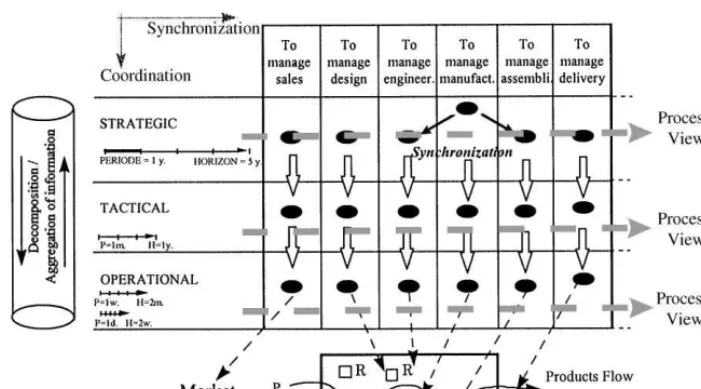
Two decomposition axes are de"ned (Fig. 1).
A vertical axis linked to the nature of decisions: The"rst criterion is a temporal one linked with the classical decomposition by level of decision: stra-tegic, tactical, operational (Fig. 1):
Strategic: the decisions which allow to de"ne the goals to achieve on one considered horizon,
Tactical: the decisions which allow to set up the resources and the products on a middle term, and Operational: decisions which allow to execute the product transformation activities by the resources on a short-term horizon.
We assign to each level a temporal characteristic:
f Horizon: The interval of time over which the
Fig. 1. The global GRAI Model for the enterprise.
f Period: The interval of time after which we
recon-sider the set of decisions. In such a structure, the horizon is sliding.
A horizontal axis linked to the nature of decisions: The second criteria of decomposition is the func-tional activities decomposition criteria.
For the enterprise, six functions are taken into account: to manage sales, to manage design, to manage engineering, to manage manufacturing, to manage assembling, and to manage delivery (Fig. 1). There can exist other functions according to the type of enterprise and the development of reference model will bring new answer to this question. The interest of this model is to facilitate the integration between decisional levels and between functions.
The matrix structure allows to co-ordinate the functional view (vertical) and the process view (horizontal) by decisional level (Fig. 1).
Moreover, there is a strong relationship between the physical system decomposition and the deci-sional levels, each level controlling a part more or less aggregated of the physical system.
A decision centre is conceptually de"ned as the cross between a function and a decision level.
There the two kinds of links between two deci-sion centres: information link (simple arrow) and decision (hierarchical) link represented by a
&deci-sion frame' (double arrow). Through the decision frame,a decision centre transmits to another decision centre the objectives, the decision variables, the criteria and the constraints that this last decision centre has to take into account in its decision.
This"rst model for the enterprise can be decom-posed more accurately by taking the basic prin-ciples of the GRAI Model into account to manage the synchronisation of activities.
At each decisional level, the performance objec-tive imposes the need to synchronise in time the product and resource availability to perform the activity with the highest level of performance.
Thus, there are three basic types of functional activities: The product management activities, the planning activities and the resource management activities (Fig. 2).
In the Fig. 2, the product management activities are linked with the purpose of the function, which is: to transform raw materials and components into "nal products according to the objectives, constraints, and criteria (optimisation of some features). We "nd in product management, the classical functions: to buy, to purchase, to store.
Fig. 2. The global GRAI Model for the control of each function.
Fig. 3. Di!erence between objective and performance indicator concepts.
The planning activities realise the synchronisa-tion between the two previous activities: a good management allows the short-term level (opera-tional level) to synchronise the available means and the products to be transformed.
To these three basic functions, we propose to add the decisional activities linked to the quality man-agement (linked to products), and to the mainten-ance management (linked to resources).
We get the grid represented in Fig. 2. This basic decomposition can be applied to each function of the global grid of Fig. 1.
By combining Figs. 1 and 2, a general grid of 6 functions]5 columns"30 columns could be built. In practice, one focuses on a main function which will depend on the studied domain, the others being represented by only one column.
4. De5nition of objectives
Based on literature survey [17}19], the following syntactic and semantic de"nition is chosen [20]:
An objective expresses the intention of going from an existing performance status to the
ex-pected performance status for the physical sys-tem controlled by a decision centre. This objec-tive must be expressed with a verb explaining the expected trend (i.e. to increase, to decrease, to maintain2) associated to a considered
perfor-mance domain (i.e. cost, quality, lead time, #exib-ility2).
So, each objective is associated to a decision centre which controls a speci"c activity to make it achieve a speci"c level of performance.
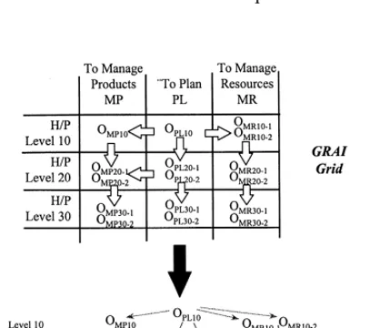
Fig. 4. The graph of decomposition.
5. Graph of a priori decomposition
5.1. Building of the graph
As it is explained above, in the GRAI Model, and particularly in the GRAI grid, the objectives are decomposed between decision centres through the decision frames.
But the decision frames are relationships be-tween decision centres and not directly bebe-tween objectives. It means that if one decision centre, containing two objectives, is related with a decision frame to another decision centre, containing also two objectives, it is not possible to know a priori the respective relationships between objectives. That is why we propose, "rst, to use a graph of decomposition to represent the a priori ships between objectives (Fig. 4). These relation-ships are elaborated according"rst to the decision frames and than to the experience of the decision makers.
Then, the coherence analysis between the objec-tives aims to verify the relevancy of each decompo-sition relationship between the objectives of the graph.
For instance, in Fig. 4, there is a decision frame between the decision centres (to manage products }Level 10) MP10 and MP20. Then, the decision makers determined there is a priori a relationship
between O
MP10 and OMP20v1 and no relationship
betweenO
MP10 and OMP20v2. The further analysis
will be able to con"rm this situation.
5.2. First analysis of the graph of decomposition
The goal of the"rst analysis of the graph is to detect if there exist objectives which are not decom-posed or which are not the decomposition of another.
In Fig. 4, the objective OMR10
v2 is not
decom-posed in another objective at the same or at the upper level of decision. It means that this objective will not be achieved by acting at the operational level.
In order to correct this incoherence, two solu-tions are proposed:
f to add an objective at the upper decision level
(MR20),
f to remove the objectiveO
MR10v2. This solution is
dangerous because this objective is the decompo-sition of O
PL10 and its removal can be fatal for
the achievement of this last objective.
6. Typology of decomposition between objectives
Based on the GRAI Model concepts and on the de"nition of objectives, the decomposition between father (i.e. superior) objective and son (i.e. inferior) objectives can have di!erent forms. The kind of decomposition between the objectives has a great in#uence in the way the coherence is analysed.
Starting from the previous de"nition, two classes of decomposition are de"ned: homogeneous and heterogeneous decomposition. These two de-compositions are explained next.
6.1. Homogeneous decomposition
Fig. 5. An example of homogeneous decomposition.
Fig. 6. Two cases of heterogeneous decomposition of objectives.
performance domains are called &reference perfor-mance domains'. We propose only three reference domains but others can be de"ned as in [21] or [22], depending on the enterprise strategy. In fact, these performance reference domains arethe perfor-mance domains of the enterprise global objectives.
The main reason for choosing the performance domains of the global objectives as reference performance domains is that these objectives are the most important for the enterprise and all the lower objectives and actions must be achieved taking these global objectives into account.
Anyway, the reference performance domains of the enterprise, even if they are di!erent than the cost, lead time and quality rate, must be able to be quanti"ed precisely in order to achieve them.
An example of homogeneous decomposition is presented in Fig. 5.
In Fig. 5, the qualitative objective at the upper level (father objective),&to decrease production cost' is the"rst objective of the decision centre PL20 (i.e. the decision centre at the cross of the function&to plan' and the decisional level no. 20 of the GRAI
Grid). This objective is decomposed in only one son quantitative objective&To decrease inventory cost by 5%'at the same level (no. 20) for the function&to manage products'. So, the performance domain is the cost for both objectives. The decomposition is then homogeneous.
6.2. Heterogeneous decomposition
The heterogeneous decomposition includes two kinds of decomposition between father and son objectives:
f either the two objectives are expressed in
di!er-ent performance domains (Fig. 6a),
f or they are expressed in the same performance
domain but this domain is not a performance reference domain (i.e. cost, lead time, or quality rate) (Fig. 6b).
In Fig. 6a, the performance domains of father ob-jective&to decrease production cost'is then the cost. The performance domain of the son objective &to de"ne several suppliers for speci"c parts' is the number of suppliers. So, the two performance domains are di!erent.
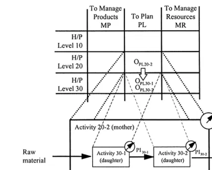
Fig. 7. Relationship between the decompositions of physical and decision systems.
Then, for each kind of decomposition, we will present a speci"c method to analyse the coherence of quantitative objectives.
7. Relationships between the decompositions of physical and decision systems
As it is de"ned previously, an objective is de"ned for a decision centre and represents the perfor-mance to achieve by the activity controlled by this centre.
In the GRAI Model, each decision level (10, 20, 30,2), controls a part more or less aggregated of
the physical system. It means that the level 10 controls the physical system in its globality although the level 20 controls a part less aggregated of this system (for instance, a speci"c shop).
Thus, if we consider a father objective, at the level 20, and a son objective at the level 30, there must exist a decomposition between the activity&mother' controlled by the level 20 and the activity &daugh-ter' controlled by the level 30 as represented in Fig. 7.
This conclusion shows that the coherence analy-sis between objectives depends strongly on the decomposition of activities they control.
In Fig. 7, the decisional level 20 controls the activity 20-2 of the physical system. The objectives of the various decision centres of the level 20 (as for instanceO
PL20v2) are assigned to this activity. The
performance of the activity 20-2 is measured with PI
20v2(but there can exist several PIs). In the same
way, the level 30 controls the detailed activities 30-1
and 30-2. So, the objectives O
PL30v1 and
O
PL30v2 can be assigned to one or both of these
detailed activities. The performance of detailed activity 30-1 is measured by PI
30v1and that of the
activity 30-2 by PI
30v2.
This"gure shows that the coherence between the objective O
PL20v2 (i.e. the performance to achieve
by the activity 20-2) and the objectivesO
PL30v1(i.e.
the performance to achieve by the activity 30-1) and O
PL30v2 (i.e. the performance to achieve by
the activity 30-2) depends on the decomposition of the detailed activities in the global activity. In the case of Fig. 7, the decomposition is sequential.
Therefore, it is necessary to ensure that all considered objectives are assigned to the activities during the exploitation phase of the manufacturing system and not during the design phase of this system
8. Typology of decomposition of physical system activities
8.1. Typology of decomposition of one activity in two detailed activities
In fact, the coherence analysis consists "rst in the aggregation of the performances related to son objectives, and assigned to detailed
activities, and in comparing the result of
this aggregation to the performance related to the father objective and assigned to the global activity.
As mentioned above, the coherence depends on the decomposition of physical system activities.
But this aggregation depends also on the performance domain which is considered. In the following, we will consider"rst only the reference performance domains, the other domains being
considered especially for the heterogeneous
Fig. 8. Sequential decomposition.
Fig. 9. OR decomposition.
Fig. 10. AND decomposition.
Fig. 11. Generalised sequential decomposition.
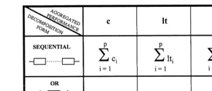
So, three kinds of decomposition between activ-ities are de"ned:
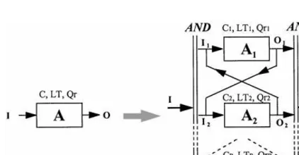
The sequential decomposition (Fig. 8):
In the decomposition of Fig. 8, the product can change activity only if the previous one is"nished. Each detailed activity has the following perfor-mances:
f forA
1:C1, LT1, Qr1, f forA
2:C2, LT2, Qr2.
The OR decomposition (Fig. 9):
In the decomposition of Fig. 9, the product can be processed either by the activity A
1 or A2, the
result of the transformation being the same, but the activities have di!erent performances in terms of cost, lead time and quality rate.
Each detailed activity has the following perfor-mances:
f forA
1:C1, LT1, Qr1, f forA
2:C2, LT2, Qr2.
The AND decomposition (Fig. 10):
By the decomposition of Fig. 10, the product can be processed simultaneously by the activities A1 andA2, the result of the transformation being considered after the two processes.
Each detailed activity has the following perfor-mances:
f forA
1:C1, LT1, Qr1, f forA
2:C2, LT2, Qr2.
8.2. Generalisation of decomposition of one activity in several detailed activities
The previous typology is interesting when one global activity is decomposed in two detailed activ-ities. In a lot of cases, one activity is decomposed in several sequential ones for instance. Nevertheless, the previous decomposition could be used several times but in order to save time in the calculus of the aggregation, we propose to generalise the previous approach for one activity decomposed in several activities. The typology is kept and three cases are then considered.
The generalised sequential decomposition (Fig. 11): In the decomposition of Fig. 11, the product can change activity only if the previous one is"nished. Each detailed activity has the following perfor-mances:
f forA
1:C1, LT1, Qr1, f forA
2:C2, LT2, Qr2, f forA
p:Cp, LTp, Qrp.
The generalised OR decomposition (Fig. 12): By the decomposition of Fig. 12, the product can be processed either by activityA
1orA2orAp, the
Fig. 12. Generalised OR decomposition.
Fig. 13. Generalised AND decomposition.
Fig. 14. Formula to aggregate the detailed performances.
Each detailed activity has the following perfor-mances:
f forA
1:C1, LT1, Qr1, f forA
2:C2, LT2, Qr2, f forA
p:Cp, LTp, Qrp.
The generalised AND decomposition (Fig. 13): By the decomposition of Fig. 13, the product can be processed simultaneously with the activities A
1,A2 and Ap, the result of the transformation
being considered after the various processes. Each detailed activity has the following perfor-mances:
f forA
1:C1, LT1, Qr1, f forA
2:C2, LT2, Qr2, f forA
p:Cp, LTp, Qrp.
8.3. Combination of the various decompositions for the representation of the physical system
Based on the previous decomposition forms, it is possible to decompose any physical system
struc-ture and to elaborate the links between the physical and the decision systems, that is, the links between the various more or less aggregated activities and the various decision centres of the GRAI grid.
9. Coherence analysis for homogeneous decomposition of objectives
After having elaborated the decomposition typology for the physical activities, it is necessary now to de"ne the aggregation formula in order to calculate the global performance of the global activity by knowing the detailed performances of the detailed activities.
These aggregation formulas depend, of course, on the decomposition but also on the reference performance domain.
Fig. 14 presents the result of aggregated perfor-mance for the mother activity according to the decomposition form and the reference performance domain.
It is necessary to mention that the formula given in Fig. 14 representsthe most pessimistic case.
It is then possible to compare this calculated global possible performance with the expected global performance (objective) and then to analyse the coherence between father and son objectives.
When the reference performance domains (i.e. those of the global objectives) are di!erent, it is necessary to establish the same formula for each new domain.
Nevertheless, the absolute coherence (no di!er-ence between possible and expected global perfor-mance) is not frequent.
That is why it is necessary to de"ne an accepted di!erence between the two results over which the objectives are not coherent.
The di!erence is equal to 10% of the perfor-mance of the father objective. When the di!erence will be less than 10%, the father and son objectives will be considered as coherent.
10. Coherence analysis for heterogeneous decomposition of objectives
This part aims at contributing to a method to analyse the coherence of objectives which are expressed in the same performance domain the later being di!erent from a reference performance domain or between objectives which are expressed in di!erent performance domains. Indeed, the per-formance domain of objectives can be completely di!erent according to the decision level. Parti-cularly, at the short-term level, they can be di!erent from the reference performance domains. First, this di!erence is due to the perception of the physical system of the decision makers. Because each deci-sion level has a di!erent view of the physical system, the decision makers have di!erent criteria to evaluate the performance of the activities they control. Moreover, for the same decision level, this di!erence exists for decision makers of di!erent functions because they do not control the same entities (resources, or products, or both).
10.1. Basis of reference domains
10.1.1. Multi-criteria analysis concepts
The basic concept of the multi-criteria analysis is, when comparing two di!erent things, to express
them on the same basis of criteria and to compare each expression on this basis.
In the state of the art, there exists a lot of math-ematical methods for mono or multi-criteria analy-sis (constrain optimisation, simplex, etc.). Nevertheless, for the qualitative problems, these methods are not adapted because they require too much information [23].
That is why it was decided to express each objec-tive on the basis of several criteria in order to compare them. These criteria are in fact perfor-mance domains in which each objective will be expressed.
10.1.2. Choice of the performance domains of the basis
The choice of the performance domains of the basis will condition further results of the coherence analysis. That is why this choice must be relevant. For the same reasons as previously, these perfor-mance domains will be the reference perforperfor-mance domains used for the coherence analysis in the homogeneous decomposition (i.e. cost, lead time and quality rate or other domains of the global objectives of the enterprise).
10.1.3. Performancevector
Each objective represents a performance to achieve. So, it can be expressed on a performance axis as explained previously.
Then, each performanceP
1(e.g. a resource
utilis-ation rate) and then each objective can be expressed with a vector with coordinatesn
11,n12, andn13, on
the basis of the three reference performance domains as presented below:
P
10.2. Normalisation coezcient
This part aims at de"ning how to calculate the various coe$cientsn
ij of the previous vector.
These coe$cients represent the relationship be-tween the considered performanceP
1and each of
Fig. 15. Decomposition of one global activity in two detailed activities.
When the performance P
1 will evolve in the
sense of the objective, then the various reference performance domains will also evolve (ifn
ijO0).
For instance, the improvement of the utilisation rate for a resource makes the cost and the lead time to evolve in relation to this resource.
It is then possible to conclude that the coe$-cients n
ij represent the ratio between variation of
the considered performanceP
1and the variation of
the reference performance.
It implies that if both performances evolve in a di!erent direction, then the coe$cient will be negative.
One can write then
n
It is possible then to explain how to calculate the various coe$cients.
Indeed, if a decision maker knows that a
vari-ation of x% of the performance P
1 makes the
reference performanceCofy%, to evolve then it is possible to calculate the coe$cients without know-ing the absolute expected performances.
It is possible to demonstrate easily that
n
In the same way, it is then possible to calculate all the coe$cients.
For instance, considering a decision centre with three objectives expressed in three di!erent
perfor-mances P
1,P2,P3, the following matrix, called
&normalisation matrix &or'matrix of coe$cients'is obtained:
Based on this matrix, one obtains for the domainc@ the relationships
c"+n
ijpi.
10.3. Example of normalisation matrix
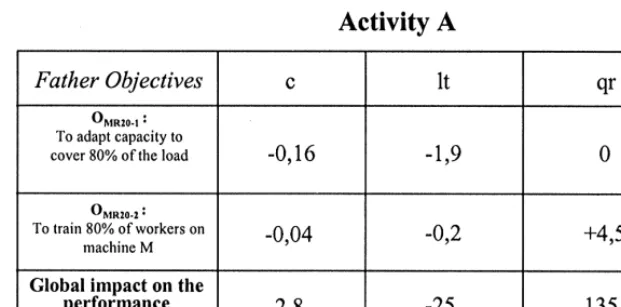
An example of controlled activities decomposi-tion is presented in Fig. 15.
Fig. 15 shows a global activity A decomposed into two detailed activitiesA
1 andA2.
The objectivesO
MR20v1andOMR20v2in charge of
the decision centre of the function&to manage re-sources'at the decision level 20, are assigned to the controlled activityA.
The objectivesO
MR30v1andOMR30v2in charge of
the decision centre of the function&to manage re-sources'at the decision level 30, are assigned to the controlled activityA
1.
The objectiveO
MR30v1andOMR30v3 in charge of
the decision centre of the function&to manage re-sources'at the decision level 30, are assigned to the controlled activityA
2.
The normalisation matrix for the activity A is presented in (Fig. 16).
The objectives of the detailed activities are
f O
MR30v1: to increase the utilisation rate of human
and technical production resources to 88%,
f O
MR30v2: to keep 10% of the capacity for load,
f O
MR30v3: to improve the quality control reaching
a quality rate of 90% for activityA
2.
The normalisation matrices for the activities A1 andA2 are presented in Fig. 17.
Now, it is necessary to de"ne the procedure to aggregate the detailed performances in order to be able to compare them with the global ones.
10.4. Matrix of contribution%
Fig. 16. Normalisation matrix for activityA.
Fig. 17. Normalisation matrices for activitiesA
1andA2.
Fig. 18. Decision frame and objective decomposition between two decision centres.
This paragraph shows the contribution of a son decision centre in the achievement of the father decision centre objectives.
By considering two decision centres CD1 and CD2 related by a decision frame, it is shown that there exists a decomposition between the objectives of CD1 and CD2 (Fig. 18).
The decision centre CD1 has a performance vari-ation vector:
p1"
C
p
11
p12 p
13
D
.
The decision centre CD2 has a performance vari-ation vector:
p
2"
C
p
21
p
22
p
23
D
.
The decision centre CD1 contributes to the im-provement of the reference performances through the matrixN
1.
The decision centre CD2 contributes to the
improvement of the reference performances
through the matrixN
2.
Fig. 19. Aggregation formula of normalisation coe$cients.
performance, it means the achievement of the objectives of CD1.
This partial contribution is formalised below. Then,
The contribution of a variation of the reference performances of CD2 &p
3%&2' to the variation of
reference performance of CD1&p
3%&1'is represented
by the contribution matrix%2,1 with
p
3%&1"%2,1p3%&2#C,
whereCis the contribution to the reference perfor-mance of the other decision centres related to CD1.
One can also write
C
cijdepend on the decomposition of
the physical activities controlled by CD1 and CD2. Actually, the coe$cients z
ij are not quanti"ed
values but operators, it means sum& or products
%. These operators can also be Min or Max
operators.
10.5. Operators of the matrix of contribution%
The concepts for the operators of the contribu-tion matrix are similar to those of the homogene-ous decomposition.
Indeed, this decomposition depends, as in the previous case on
f the control links, and then the assignment of
each objective to a part of the physical system,
f the kind of decomposition of physical activities.
One could think"rst that the aggregation formula is the same as previously but one distinction is important.
Previously, for the homogeneous decomposition, the formulas are absolute values of performances expressed in particular units.
In the current case, the coe$cients of normalisa-tion are without unit because they are rates of variations. That is why the formulas for the homo-geneous decomposition are not valid for the contri-bution matrix%.
By elaborating, for each kind of decomposition of physical activities, the formula for the perfor-mance aggregation, we obtain the formula of Fig. 19.
The operators in the"gure above are then placed in the contribution matrix, depending on the de-composition form between the activities controlled by CD1 and CD2 and on the reference perfor-mance.
10.6. Example of performance aggregation and comparison
Fig. 20. Result of the aggregation in the case of Section 10.3.
Fig. 21. Comparison between the aggregated expected perfor-mances of detailed activities (son objectives) with those expected for the global activity.
As for the homogeneous decomposition, the absolute coherence does not exist, and we de"ne an accepted di!erence between the two results over which the objectives are not coherent.
The di!erence is equal to 10% of the normalisa-tion coe$cients of father objective. When the di!er-ence will be less than 10%, the father and son objectives will be de"ned as coherent.
The result of the comparison is presented in Fig. 21.
In this case, the di!erence being less than 10% of the father objectives, the son objectives are then coherent with the father ones.
11. Conclusion
This paper presents a method to analyse the coherence in the decomposition of quantitative objectives.
This method is based on the decomposition of physical activities on which are assigned the vari-ous objectives.
An example is presented in order to illustrate the application of the method in the case of heterogen-eous decomposition.
This example shows that the coherence analysis requires many pieces of information concerning the quantitative expected performances of each con-trolled activities. This information is often di$cult to obtain but their de"nition and their collection is essential in order to de"ne clearly the evolution of the system.
When the decision makers cannot give precise quantitative objectives, it is necessary to analyse also the coherence. So, the next step of our research work is to elaborate a method for the coherence analysis of qualitative objectives.
References
[1] M. Porter, L'avantage concurrentiel}comment devancer ses concurrents et maintenir son avance, Inter Editions, 1986, 643p.
[2] J.P. Womack, D.T. Jones, D. Roos, The System that Changed the World, MIT Rawson Associates, Cambridge, MA, 1990.
[3] S.M. Hronec, Vital signs: Des indicateurs cou(ts, qualiteH, deHlais pour optimiser la performance de l'entreprise, Les eHditions d'Organisation, August 1995, 255pp.
[4] A.D. Neely, Performance measurement system design, Theory and Practice, Manufacturing Engineering Group, University of Cambridge, April 1993.
[5] A. Neely, J. Mills, M. Gregory, H. Richards, K. Platts, M. Bourne, Getting the measure of your business, Depart-ment of Trade Industry, Engineering and Physical Sciences Research Council, Published by Work Manage-ment, University of Cambridge, 1996.
[6] M.W. Grady, Performance measurement, Implementing Strategy, Management Accounting (1991) 49}53. [7] R.S. Kaplan, D.P. Norton, Translating Strategy into
Action } The Balanced Scorecard, Harward Business School Press, Boston, MA, 1996.
[8] G. Doumeingts, B. Vallespir, D. Chen, GRAI grid, deci-sional modelling, in: P. Bernus, K. Mertins, G. Schmith
(Eds.), Handbook on Architecture of Information System International Handbook on Information Systems, Springer, Berlin, 1998.
[9] J.C. Hennet, Concepts et outils pour les syste`mes de production, CeHpadues Editions, April 1997, 325pp. [10] M.C. Rousset, Sur la coheHrence et la validation des bases
de connaissances: Le syste`me COVADIS, The`se de docteur d'eHtat, UniversiteH de Paris Sud, Centre d'Orsay, 1988.
[11] J.L. Ermine, Syste`mes experts: TheHorie et pratique, Tech-nique et documentation, Lavoisier, 1989.
[12] M. Ayel, B. Wendler, Verifying coherence in modular KBSs', EUROVAV-95 Chambery, 1995, pp. 173}188.
[13] Y. Ducq, Contribution a` l'analyse de la coheHrence des structures de production par le mode`le GRAI: Application au projet I.M.S. Globeman 21, MeHmoire de DEA, Produc-tique, UniversiteH Bordeaux I, September 1993.
[14] A.H. Bond, Distributed decision making in organisation, IEEE Transactions on Systems, Man and Cybernetics Conference, November 1990.
[15] H.J. Warnecke, The Fractal Company, Springer, Berlin, 1993.
[16] A. Tharumarajah, A.J. Wells, L. Nemes, Comparison of the bionic, fractal and holonic manufacturing system con-cepts, Computer Integrated Manufacturing 9 (3) (1996) 217}226.
[17] J. Melese, L'analyse modulaire des syste`mes de gestion, Editions Hommes et Techniques, 1972.
[18] M.D. Mesarovic, D. Macko, T. Takahara, Theory of Hier-archical, Multilevel Systems, Academic Press, New York, 1970.
[19] P. Lorino, Comptes et reHcits de la performance: Essai sur le pilotage de l'entreprise, Les EDditions d'Organisation, June 1995, 288pp.
[20] Y. Ducq, Contribution a` une meHthode d'analyse de la coheHrence des syste`mes de production dans le cadre du mode`le GRAI, The`se de doctorat de l'UniversiteH de Bordeaux I, 1999.
[21] D.A. Garvin, Manufacturing strateHgic planning, California Management Review (Summer) (1993) 85}106.
[22] B.M. Kleiner, An integrative framework for measuring and evaluating information management performance, Computer Industrial Engineering 32 (3) (1997) 545}555. [23] J.C. Pomerol, S. Barbara-Romero, Choix multicrite`re dans