Comparative Study of Equivalent Manning Roughness
Coefficient for Channel with Composite Roughness
Djajadi, R.1
Abstract: This paper reviews the applicability of nine selected expressions in determining the equivalent value of the Manning coefficient of roughness. For this purpose, a prismatic 4m-long and 0.05m-wide trapezoidal-shape channel was constructed, namely the homogeneous channel and the composite channel. The homogeneous channel had the same surface lining, whereas the composite channel had two different surface linings. Four different lining materials were considered: plaster, small, medium, and large-sized aggregates. The homogeneous channel showed a reliable Manning coefficient prediction, provided that a uniform flow was achieved. The roughness of the composite channel can be predicted accurately by the nine expressions; the average was 0.96, with standard deviation of 11.13%. Out of the nine expressions, the expression that considers wet-perimeter as its main parameter showed the best estimate. The error was about 2% with standard deviation of 5.15%. This can be actually traced back to the limited width of the test channel, thereby increasing the role of wet perimeter.
Keywords: manning coefficient, open channel, uniform flow, composite roughness
Introduction
Water flowing in an open channel runs in relatively complex manner due to various influencing factors, including slope steepness, surface roughness, and the so-called hydraulic radius. The Manning equation [1], which was introduced about a century ago, attempts to capture the essential features of these factors. This empirical equation offers a simple yet reliable expression and indeed has a physical meaning rooted in it. Accordingly, the average velocity at a given open-channel section v can be simply related to the abovementioned factors in the following equation:
2 1 3 2
1
S
R
n
v
=
×
×
(1)where n is a parameter that indicates the friction provided by channel lining, the so-called Manning coefficient of roughness, R the hydraulic radius (in m unit), and S the channel gradient.
Despite the straightforwardness of the Manning equation, one difficulty arises in determining the Manning coefficient n.
1
Email: [email protected]
Civil Engineering Department, Faculty of Civil Engineering and Planning, Petra Christian University. Siwalankerto 121-131, East Java, Indonesia
Note: Discussion is expected before November, 1st 2009, and will be published in the “Civil Engineering Dimension” volume 12, number 1, March 2010.
Received 7 November 2008; revised 10 February 2009; accepted 3 April 2009.
Unlike the other two factors (R and S), which can be quantitatively measured, the n value has to be determined rather qualitatively. In principle, it depends on the characteristic of run-off surface. The rougher the surface, the larger the n value, and hence the slower the resulting average water velocity v is. For instance, a channel with concrete lining would yield an n-value of approximately 0.015, whilst one with gravel lining would correspond to about 0.020. These factors are available in many literatures [2, 3]. The selection of n value would consequently not pose a significant problem, provided that a comparable roughness of channel lining exists.
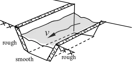
v
roughsmooth rough
Figure 1. Illustration of a composite channel
Fortunately, a number of rather diverse expressions exist to estimate the average roughness of open channel, an equivalent Manning coefficient ne [2, 4, 5]. Nevertheless, as the expressions were derived from various fundamental assumptions, it can be said that one expression will more suit to a certain situation, and less to others.
The objective of this paper is therefore to conduct a comparative study on the applicability of several expressions in calculating ne, as no direct comparisons have been yet undertaken. A prismatic open channel was accordingly constructed in which the surface was varied as the primary experiment variables. Two channel types were made: a homogeneous channel, which had a uniform lining material, and a composite channel, which had two combination lining materials.. The former was intended to verify the accuracy of the experiment devices, while the later was designed to study the effects of different lining surface.
Attention was given to the differences between the measured and the predicted ne
Material Type
values
Literature Review
Manning Coefficient
The characteristic of channel-lining surface can be used as an indicator that control the velocity of water flow. Apart from its roughness, different material type also yields different value of n value. A typical n value is given in Table 1.
Table 1. Typical Value of Manning Coefficient of Roughness [2]
ManningCoefficient n
Soil 0.025
Concrete 0.015
Gravel 0.020
Wood 0.013
Flat steel 0.012 Corrugated steel 0.025
Glass 0.010
Equivalent Manning Coefficient
Many expressions are currently available to be used to estimate the average roughness of a given open channel, which commonly known as the equivalent Manning coefficient ne
(
)
3. The author would recall nine distinguished expressions, which hereafter designated as Expression 1 to 9; three are picked up from Ref. 2, two from Ref. 4, and the other four from Ref. 5. These nine expressions are listed as follows:
- Expression 1
The expression shown in Eq. 2 was originally proposed by Horton [6] and Einstein [7]. The core assumption of this expression is that, at any given section of a channel, the average velocity always equals to the corresponding total average velocity.
(2)
- Expression 2
This expression was intensively used by Pavlovskii [8], Muhlhofer [9], Einstein & Banks [10]. It is assumed that total resistance force equals to the sum of all resistance forces in each section. This assumption yields the following:
(
)
2In 1993, Lotter [11]derived the ne value based on the assumption of the equality of total discharge to the sum of all discharge of each section. The prediction of ne
Another simplified relationship was proposed by Cox [12] as follow:
In the same year, he also proposed another simplified expression, designated in this paper as Expression 5. The expression is known as Colebatch Method [12] and is given as shown in Equation 6 .
- Expression 5
The next four expressions are taken from Soong and Hoffmann [5]
- Expression 6
(
)
3 1i 3 1 i i e
R
P
n
R
P
n
=
∑
(7)- Expression 7
This expression commonly known as shear force II method. The approximate value of ne
(
)
6 1
i 6 i i e
R
P
n
R
P
n
=
∑
is given by
(8)
- Expression 8
In 1960, Felkel used the following expression to obtain the value of ne
∑
=
i i e
n
P
P
n
as given by:
(9)
- Expression 9
This last expresion is based on the assumption of component roughness is linearly proportional to wetted perimeter. The expression is given as
P
n
P
n
ii
e
∑
=
(10)Uniform Flow
It is important, for simplicity, to ensure a uniform flow distribution while using the Manning equation (Eq. 1). The term uniform here means that the fluid velocity has to be the same magnitude and direction at any points. To ensure the uniformity of the flow, the energy gradient, the water-surface gradient, and the channel slope have to be paralell to each other (see Fig. 2). This can be found, for instance, in an infinitely long straigth channel, with a similar depth and cross-sectional area (e.g.: prismatic channel).
energy gradient
water-surface gradient
channel slope
v
2/2g
y
Figure 2. Illustration of uniform flow
(a)
(b)
Channel s
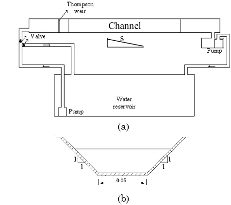
Figure 3. Schematic of the test channel: (a) General overview, (b) Typical cross section of the channel
Table 2. Experiment variables
Case Lining Surface Material Remarks
Bottom Surface Sidewalls
1 P P
Homogeneous Channel
2 SA SA
3 MA MA
4 LA LA
5 P SA
Composite Channel
6 P MA
7 P LA
8 SA LA
Note:
P: Plaster; SA: Small-sized aggregate (2-3 mm); MA: Medium-sized aggregate (7-10 mm); LA: Large-sized aggregate (12-17 mm).
Experimental Program
General Overview
The experimental program involved the testing of a laboratory-scale channel with various channel lining roughness. The schematic of the channel is shown in Fig. 3.
The channel was 4 m long and 0.05 m wide with a typical cross section as shown in Fig. 3(b). The side wall of the channel was made 45o inclined (z = 1). The longitudinal gradient of the channel S was fixed at 0.005.
Construction of the channel
The channel was made of bricks, with various finishing materials as listed in Table 2. The plaster (P) was made of mortar with cement and sand ratio of 1:3. To obtain a smooth surface, a cement paste was applied as the finishing surface. For the case with aggregate, the channel was first plastered and the aggregate was then attached manually by hand.
Results and Discussions
Homogeneous Channel
The equivalent Manning coefficient ne of the homogeneous channel, which was computed based on the Manning equation (Eq. 1), is shown in Fig. 4. Also shown in the figure is the reference values previously listed in Table 1.
The obtained values are in a good aggrement with the reference ones, provided that a uniform flow of water was achieved. It is very evident as the finishing surface of the channel became rougher, the n value increased. The smallest n value was 0.0136, corresponding to a channel with plaster finishing, the smoothest surface finishing tested herein. This value implied that the roughness of the plaster surface was somewhat inbetween wood and concrete. The largest n value was 0.0286 and belonged to a channel with large-sized aggregate (LG). This value was even larger than those of stone and soil. The protuding aggregates from the channel surface was most likely the potential factor for this substantial increase as the aggregate size was comparatively large compared to the width of the channel.
Figure 4. Comparison of the obtained and the reference n
values for homogeneous channel. (Note: solid circles are the obtained values).
Composite Channel
Employing a similar procedure likewise in the homogeneous channel, the ne value of the composite channel is listed in Table 3. The ratio of the ne
Method
values
predicted by the nine expressions to the ones observed from the expreiment is shown in Fig. 5.
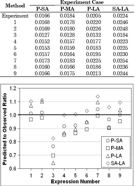
Table 3. Equivalent Manning Coefficient of Composite Channel (Experiment)
Experiment Case
P-SA P-MA P-LA SA-LA
Experiment 0.0166 0.0184 0.0205 0.0224 1 0.0168 0.0178 0.0220 0.0246 2 0.0169 0.0180 0.0226 0.0248 3 0.0127 0.0128 0.0132 0.0184 4 0.0152 0.0157 0.0177 0.0223 5 0.0153 0.0159 0.0183 0.0225 6 0.0157 0.0164 0.0195 0.0230 7 0.0173 0.0183 0.0225 0.0254 8 0.0160 0.0166 0.0186 0.0236 9 0.0166 0.0175 0.0213 0.0244
Figure 5. Predicted to Obtained ne values of composite channel
In general, the predicted values were fair enough, although some entries were rather erratic (particularly those obtained from Expression 3). Some entries matched with the observed value at their lower bound (e.g.: Expression 1, 2, 7, and 9), and some others at their upper bound (e.g.: Expression 4, 5, 6, 8). This means the former group would be more accurate in estimating the equivalent roughness ne of a channel with smooth bottom surface and slightly coarser sidewalls. On the other hand, the later group can serve a better estimation in the case of a waterway with slighly rough bottom surface and much rougher sidewalls.
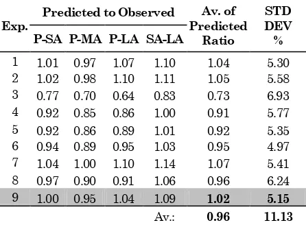
Table 4. Ratio of Predicted to Observed ne
Exp.
values of Composite Channel
Predicted to Observed Av. of Predicted
Ratio
STD DEV % P-SA P-MA P-LA SA-LA
1 1.01 0.97 1.07 1.10 1.04 5.30 2 1.02 0.98 1.10 1.11 1.05 5.58 3 0.77 0.70 0.64 0.83 0.73 6.93 4 0.92 0.85 0.86 1.00 0.91 5.77 5 0.92 0.86 0.89 1.01 0.92 5.35 6 0.94 0.89 0.95 1.03 0.95 4.97 7 1.04 1.00 1.10 1.14 1.07 5.41 8 0.97 0.90 0.91 1.06 0.96 6.24 9 1.00 0.95 1.04 1.09 1.02 5.15
Av.: 0.96 11.13
The accuracy of Expression 9 (Eq. 10) implies that the so-called wet perimeter was the governing factor in determining the value of ne. Meanwhile, the other methods were less accurate as they used different parameters such as cross-sectional area, hydraulic radius, velocity, etc.
Conclusions
The Manning equation offers a simple and straigforward method in open channel flow. One of difficult parts in using this equation is in determining the so-called equivalent surface roughness coefficient ne
1. The equivalent Manning coefficient n
. Diverse provedures currently available to estimate this coefficient, but its reliability is still unrevealed. For this purpose, two types of channel was constructed: the homogeneous channel and the composite channel. Primary variables were the lining roughness that were made of plaster (P), small- (SA), medium- (MA), large-sized aggregate (LA), and the combinations of SA, P-MA, P-LA, and SA-LA. The following conclusion are drawn:
e
2. The effectiveness of nine selected procedures in determining the equivalent Manning roughness coefficient was verified. In general, all procedures could come up to a value nearly to that observed in the experiment. Only in one procedure was the estimate rather low, with 30% deviation. The overall estimated value lies at 0.96, with 11.13% deviation.
of the homogeneous channel corresponds well with the values available in literatures, provided a well-designed experimental setting was achieved. This accomplishment was primarily due to the uniformity of water flow, as designed.
3. The so-called “component roughness is linearly proportional to wetted perimeter method” expression was the one that always gave the best estimate in which the average error was just
about 2% with average standard deviation of 5.15%.
The accuracy of the aforementioned procedure can be actually traced back to the scale of test channel presented here in which the width was limited. This was intentionally decided to have a relatively long channel, and hence ensuring the uniformity of flow. This width limitation however had increased the role of the wet perimeter of the channel. Consequently, the procedure employed wet parameter as its main parameter gave the best estimate.
References
1. Manning, R., On the Flow of Water in Open Channels and Pipes, Transactions of the Institution of Civil Engineers of Ireland, Vol. 20, 1891, pp. 161-207.
2. Chow, V. T., Open-Channel Hydraulics, McGraw-Hill, New York, June 1985.
3. French, R. H., Open-Channel Hydraulics, McGraw-Hill Inc., US, Jan. 1985.
4. Stephenson, D., Stormwater Hydrology and Drainage, Development in Water Science, Vol. 14, Elsevier, Amsterdam, 1981, pp. 276-287.
5. Soong, T. W. and Hoffman, M. J., Effects of Riparian Tree Management on Flood Conveyance Study of Manning’s Roughness in Vegetated Floodplains with an Application on the Embarras River in Illinois, Contract Report 2002-02, Illinois State Water Survey Watershed Science Section Champaign, Illinois, Feb. 2002.
6. Horton, R. E., Separate Roughness Coefficients for Channel Bottom and Sides, Engineering New Record, Vol 111, No. 22, Nov. 30, 1933, pp. 652-653.
7. Einstein, H. A., The Hydraulic Cross Section Radius, Schweizerische Bauzeitung, Vol. 103, No. 8, 1934, pp. 89-91.
8. Pavlovskii, N. N., On a Design Formula for Uniform Movement in Channel with Nonhomogeneous Walls, Transactions of All-Union Scientific Research Institute of Hydraulic Engineering, Vol. 3, 1931, pp. 157-164.
9. Muhlhofer, Roughnesss Investigations in a Shaft with Concrete Bottom and Unlined Walls, Wasserkraft und Wasserwirtschaft, Vol. 28, No. 8, 1933, pp. 85-88..
11. Lotter, G. K., Considerations on Hydraulic Design of Channels with Different Roughness of Walls, Transactions of All-Union Scientific Research Institute of Hydraulic Engineering, Vol. 7, 1932, pp. 55-88.
![Table 1. Typical Value of Manning Coefficient of Roughness [2]](https://thumb-ap.123doks.com/thumbv2/123dok/3672563.1469747/2.595.59.281.532.647/table-typical-value-manning-coefficient-roughness.webp)