OCCUPANCY MODELLING FOR MOVING OBJECT DETECTION FROM LIDAR
POINT CLOUDS: A COMPARATIVE STUDY
W. Xiaoa∗, B. Valletb, Y. Xiaoc, J. Millsa, N. Paparoditisb
a
School of Engineering, NEOlab, Newcastle University, Newcastle upon Tyne, UK - [email protected] b
Universit´e Paris-Est, LaSTIG MATIS, IGN, ENSG, Saint-Mand´e, France
cDepartment of Civil and Environmental Engineering, University of Michigan, Ann Arbor, USA
Commission II, WG II/3
KEY WORDS:Laser Scanning, Change Detection, Dynamic Scene, Occupancy Grid, Probability, Dempster-Shafer Theory
ABSTRACT:
Lidar technology has been widely used in both robotics and geomatics for environment perception and mapping. Moving object detection is important in both fields as it is a fundamental step for collision avoidance, static background extraction, moving pattern analysis, etc. A simple method involves checking directly the distance between nearest points from the compared datasets. However, large distances may be obtained when two datasets have different coverages. The use of occupancy grids is a popular approach to overcome this problem. There are two common theories employed to model occupancy and to interpret the measurements, Dempster-Shafer theory and probability. This paper presents a comparative study of these two theories for occupancy modelling with the aim of moving object detection from lidar point clouds. Occupancy is modelled using both approaches and their implementations are explained and compared in details. Two lidar datasets are tested to illustrate the moving object detection results.
1. INTRODUCTION
Laser scanning, also referred to as lidar (light detection and rang-ing), has been used in both robotics and geomatics for slightly different purposes. In robotics, it is initially used for environ-ment perception to avoid collision. Nowadays, it is widely used for autonomous navigation and SLAM (simultaneous localization and mapping) (Wolf and Sukhatme, 2004; Moosmann and Stiller, 2013), so that a robot will know exactly where it is, even in a new environment. In geomatics, mapping is usually the primary goal, and laser scanning can provide a precise way of mapping the environment (Aijazi et al., 2013; Zhou and Vosselman, 2012). There are specific laser scanners for precise and dense mapping, for both indoor and outdoor, that can be operated from different platforms such as aircraft, mobile vehicles, and terrestrial tripods. One type of laser scanner that has been adopted in both robotics and geomatics studies is the Velodyne HDL-64E, which consists of 64 laser rays rotating rapidly around the vertical axis so that the surroundings are continuously scanned. Continuous scanning is essential in robotics as a robot needs toseethe environment all the time. This type of real-time laser scanner has been widely used for autonomous driving and environment mapping (Moos-mann and Stiller, 2011; Hornung et al., 2013).
Moving object detection and tracking is an important research topic for both robotics and geomatics (Lindstr¨om and Eklundh, 2001; Kaestner et al., 2012; Xiao et al., 2016). For the former, a robot, such as an autonomous vehicle needs to not only see its sur-roundings, but also make sure its trajectory will not coincide with other moving objects in a dynamic environment. Therefore, it is necessary to track and even predict other moving objects to avoid any potential collision. As for the latter, the static environment is of primary interest for mapping purposes. So moving object de-tection and removal will help clean the environment and reduce the data storage (Vallet et al., 2015). There are often movable
∗Corresponding author
objects that remain static in the data during the process of data acquisition, such as parked cars along the street. In such cases, detected moving objects can serve as training samples for com-prehensive and fully automatic mobile object removal. Moreover, object moving patterns, such as pedestrian trajectories in a pub-lic space or vehicle movement in a congregated crossroads, are potentially valuable geoinformation for further studies.
There are various methods for moving object detection from both robotics and geomatics. For example, a straightforward method is calculating the point to point distance between two different point clouds (Girardeau-Montaut et al., 2005; Xu et al., 2013; Linden-bergh and Pietrzyk, 2015), which can be two different scans. As for a real-time laser scanner, a scan refers to a full 360◦rotation of the scanner. Apart from simple point to point distance, there exist improved variants such as computing the distance between a point and a local surface, either a plane or a triangle gener-ated from local neighbour points. This method is simple and fast and still used in many applications. However, it is not able to distinguish points on moving objects from points that have no correspondence, which happens when two scans do not cover the same space, such as in occlusions. In both cases, these point will have large distances indicating movements. Another method, oc-cupancy grids, has been used initially in robotics for environment perception (Collins, 2011; Vu et al., 2011; Thrun, 2002), and re-cently in geomatics for change detection (Hebel et al., 2013; Xiao et al., 2015). It models the occupancy information of the space, i.e. whether a specific location (often a grid cell in 2D) is occu-pied by an object or not. This information is derived from the measured environment data. The occupancy states will vary by time in a dynamic environment. One of the advantages is that it is able to capture cells that have no correspondence, as all cells will be initiated but those will not be compared or updated.
Then Bayes’ rule is used to interpret measurements and update the probability (Thrun, 2002; Collins, 2011; Vu et al., 2011; Hor-nung et al., 2013). Another common approach is the Demspter-Shafer theory (DST) (Demspter-Shafer, 1992), an evidence theory that com-bines evidence from different sources and reaches a certain de-gree of belief (Murphy, 1998; Grabe et al., 2009; Delafosse et al., 2007; Moras et al., 2015; Dezert et al., 2015). There are other oc-cupancy modelling methods such as fuzzy logic (Payeur, 2003), but the former two are mostly widely used for occupancy mod-elling and moving object detection or change detection. This pa-per will investigate in detail the two methods in terms of both theory and implementation. This comparison will help the users to select the appropriate approach for their specific applications.
2. METHOD
In this section the occupancy of a laser scan is modelled using both Dempster-Shafer theory (DST) and probabilistic model ap-proaches. The occupancy definition is introduced first, then their occupancy information is fused, followed by the identification of the occupancy consistency between multiple scans.
2.1 Occupancy Definition
2.1.1 Occupancy by Dempster-Shafer theory Theoreti-cally, the space can be eitheroccupiedorfree, which are the two occupancy states. Based on DST, the occupancy is defined by the universal setX ={f ree,occupied}. And the power set ofX, 2X=
{∅,{f ree},{occupied},{f ree,occupied}}, which con-tains all the subsets ofX. In practise, if an area is not measured, there is zero knowledge about the occupancy state, meaning the occupancy isunknown. Then the space can be eitherfreeor occu-pied, so the subset{f ree,occupied}in the power set represents theunknownsituation. The DST is defined as follows:
M: 2X→[0,1], M(∅) = 0, X A∈2X
M(A) = 1 (1)
in whichM(A)is the occupancy function, including the three oc-cupancy states, namely freeM(f), occupiedM(o)and unknown M(u). They are in the range of [0, 1], and their sum equals to 1.
The occupancy needs to be modelled in 3D for the 3D laser scan-ning measurements. Along the direction of a laser rayr, the oc-cupancy is modelled in the following way. The laser ray travels through the space and is then reflected back from an object where a point is defined. So it is known to be free between the laser scanner center and the point,fr = 1;or = 0. At the location of the point, an object is supposed to be present, thus it is certainly occupied,fr= 0;or= 1. Behind the point, or ahead of the point along the ray, the space is not measured so its occupancy state is unknownur = 1. As an object will definitely be larger than a single point, the space behind the point can be assumed to be oc-cupied within a certain range. Beyond that range, the occupancy will become completely unknown. The occupancy modelling is illustrated in Figure 1.
Xiao et al. (2015) modelled the maximum occupancy slightly be-hind the point as it was argued that the point is on the surface of an object, then considering uncertainties, it can be on either side of the surface. Thus the occupancy is actually halffreeand half occupiedat this very location. By convolving with an uncertainty Gaussian function, the maximum ofoccupiedis slightly behind
0 r
Occupancy
f u
o
1
Laser Center
Figure 1. Occupancy in ray direction
the point, which is true since the space is more certain to be oc-cupied behind the surface. In this way, the occupancy along the ray is accurately modelled. However, the occupancy consistency assessment is then complicated as this will end up with half con-sistent and half conflicting for two points at the same location (see Section 2.3.1). So the maximum occupancy at the location of the point is modelled as shown in Figure 2.
0 r
Occupancy
fr ur
or 1
Laser Center
Figure 2. Occupancy in ray direction considering uncertainties
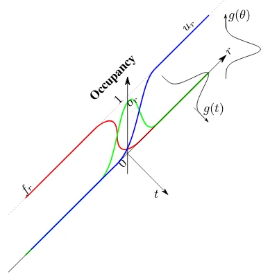
Now, the occupancy has been defined only in the ray direction. In 3D, the occupancy around a laser ray can be extrapolated to a certain extent based on the distance to the ray itself. To facilitate the extrapolation, the distance to a laser ray can be computed in the laser scanner’s own local coordinate system. Here, it is composed of the vertical angular directionθ, trajectory direction t, and the ray directionr. The occupancy is at a maximum along the ray, and it decreases along the other two directions. The 3D occupancy modelling is depicted in Figure 3.
0
r
Occupancy
fr
ur
or 1
g(θ)
g(t)
t
Figure 3. Occupancy in 3D considering uncertainties
overall occupancy of a point is a function of the three variables,
in whichgθ, gt∈[0,1]are interpolation coefficients.
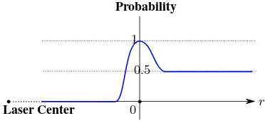
2.1.2 Probabilistic Occupancy The principle of probabilis-tic occupancy is similar to DST, where space isfreealong the laser beam andoccupiedat the location of the laser point. The probabilityP ∈ [0,1] represents the status of occupancy, i.e. P = 1when the space isoccupied,P = 0when it isfree. Fig-ure 4 shows the definition of probabilistic occupancy.
0 r
Probability
1
Laser Center
0.5
Figure 4. Probabilistic occupancy in ray direction
From the laser scanner center to the point, the laser beam has travelled through the space that is free, hence the probability is 0. At the location of the point, the space is occupied. Due to laser range measurement errors and positioning errors from the map-ping system, the point position has certain degree of uncertainty, which can be accounted for by coupling a random error distribu-tion to the probability both behind and ahead of the point along the ray direction. Further ahead of the point along the ray, the space is not scanned hence can be either free or occupied. Then the probability of occupancy is defined as 0.5. Different from DST, the probabilistic occupancy only has one value to represent the space’s occupancy status.
2.2 Occupancy Fusion
The space will be scanned multiple times by the laser scanner, meaning there will be multiple measurements at the same loca-tion. The probabilities of different scans need to be fused for final inference. This section will discuss and compare the two occupancy fusion methods.
2.2.1 Dempster’s Rule of Combination After defining the occupancy functionM(A)based on DST, the occupancy of dif-ferent rays can be fused by the Dempster’s rule of combination which is as follows: between these two setsK=P
B∩C=∅(M1(B)·M2(C)).
One important character of Dempster’s combination rule is that it is commutative and associative, meaning the occupancy from different rays can be combined in any order. For this reason other combination rules are not chosen, such as Yager’s rule which is not associative (Yager and Liu, 2008). GivenInumber of neigh-bouring raysRi, the overall occupancy is:
M(A) = ⊕
i∈I
M(A, Ri) (5)
2.2.2 Probability Interpretation and Log-odd Simplification Similarly, a location in the space can be scanned multiple times, then the probability of this location has to be updated. So the objective is to estimate the posterior probability of occupancy P(m|z1:t) of each locationmgiven the measurementsz1:t =
This gives the probability of being occupied, then the probability of being freeP( ¯m) = 1−P(m). Then,
P( ¯m|z1:t) =
P( ¯m|zt)P(zt)P( ¯m|z1:t−1)
P( ¯m)P(zt|z1:t)
(7)
By dividing Equations 6 and 7, some terms are eliminated (Thrun, 2002).
Given a probabilityP(m), the odds is defined asodds(m) = P(m)/(1−P(m)), and the logarithm log-odds is L(m) =
log( P(m)
1−P(m)). Then Equation 8 can be rewritten as:
L(m|z1:t) =L(m|zt)−L(m) +L(m|z1:t−1) (9)
Here,P(m)is the prior occupancy probability which is set to0.5 representing an unknown state, thenL(m) = 0, so
L(m|z1:t) =L(m|zt) +L(m|z1:t−1) (10)
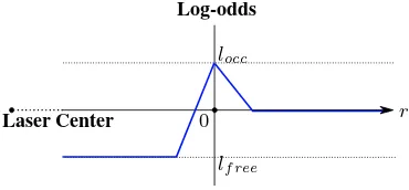
ProbabilityP ∈ [0,1]and log-odds ∈ [−∞,+∞]. Note that the occupancy probability can easily be transferred to a log-odds value, and vice versa. Due to uncertainty,P will hardly reach 1, and hence its log-odds will not be∞. In practice, log-odds values,loccandlf reeare defined to represents the occupied and free states of a single measurement. So Figure 4 is transformed to log-odds domain as shown in Figure 6.
0.2 0.4 0.6 0.8
−6
−4
−2 0 2 4 6
P
Log-odds
lmax
lmin
Figure 5. Log-odds of probability in the domain of -6 to 6
Given a laser beam, the occupancy islf reefrom the laser scanner center and increases toloccat the location of the point. To sim-plify the log-odds function for a laser beam, the transition from free to occupied is set to be linear, as also the case for the transi-tion to unknown, whereloccis decreased to 0 (Figure 6).
0 r
Log-odds
Laser Center
locc
lf ree
Figure 6. Log-odds in ray direction
For multiple measurements at the same location, their log-odds values are simply summed. Based on the definition, it can be ob-served that to change an occupancy state, it needs at least the same number of observations that define its current state. It means that if a location is consolidatedntimes by laser beams as free, anotherntimes of occupied measurement will be needed before identifying the location as being occupied. In a dynamic environment, an object will move into a free space and leave im-mediately after, depending on its speed of movement. To capture this kind of rapid change, a clamping threshold is defined to up-date the occupancy states (Yguel et al., 2007). Once the log-odds value reaches a threshold, either lower boundlminorlmax, the space occupancy state will no longer be updated. Solminorlmax are thresholds where the space is inferred as free or occupied (red in Figure 5).
2.2.3 Comparison between Dempster’s Rule of Combina-tion and Bayes’ Rule Defined by DST, space occupancy M(A)can have three states, freeM(f), occupiedM(o), and unknownM(u), and the sumPM(A) = 1
. By the proba-bilistic model, the space only has two occupancy states, either freeP(f)or occupiedP(o), and their sum also equals 1, mean-ingP(f) = P(¬o) = 1−P(o). For where the occupancy is unknown, the space is defined as half-free and half-occupied, P(f) =P(o) = 0.5.
To fuse multiple measurements, Dempster’s rule of combination
is as given in Equation 3. Bayes’ rule for an event of combined probability is as follows:
P(A|B) = P(B|A)P(A)
P(B|A)P(A) +P(B|¬A)P(¬A) (11)
In the case of probabilistic occupancy, the combined probability of two rays will be
P(o12) =
P(o1)P(o2)
P(o1)P(o2) +P(e1)P(e2)
(12)
For DST, according to Equation 3, the mass of occupied is
M(o12) =
M(o1)M(o2) +M(o1)M(u2) +M(u1)M(o2)
1−M(o1)M(e2)−M(e1)M(o2)
(13)
In case ofM(u) = 0, the equation will become
M(o12) =
M(o1)M(o2)
M(o1)M(o2) +M(e1)M(e2)
(14)
which is essentially the same as Equation 12. So, for locations whereM(u) = 0, meaning whenever there is information of oc-cupancy, the two theories, DST and Bayes’ rule, give the same result. The space between the laser scanner center and the point, in other words, the space scanned by the laser should have sim-ilar occupancy results from these two theories. However, due to uncertainties, M(u)will hardly be exactly 0. Therefore, in reality, some differences are expected. Behind the point when M(o) = M(u) = 0.5, given two similar laser rays, the com-bined occupancyM(o12) = 0.75, whereasP(o12) = 0.5. So
the occupancy evidence can still be accumulated behind the point. The DST is able to distinguish half free half occupied and half occupied half unknown, whereas the Bayes’s rule cannot.
2.3 Consistency Assessment
After combining occupancy from different rays within one scan, occupancies from different scans can be compared. This section assesses the consistency between scans to find out points on mov-ing objects.
As occupancy is often modelled in 3D voxels (Hebel et al., 2013), the consistency can be easily assessed on each voxel. However, the voxelization of the 3D space can be computationally expen-sive. A better approach is to perform the assessment directly on each individual points without voxelization. Point-level consis-tency assessment is performed for each of the occupancy mod-elling method.
2.3.1 Dempster-based Consistency The occupancy consis-tency is defined as conflicting when one scan isemptyand the other scan isoccupiedor vice versa, consistent when they have the same occupancy state, and uncertain if one dataset isunknown whereas the other one is known. The consistency relations be-tween two scans, (F1,O1,U1) and (F2,O2,U2), are defined as:
Conf lict Consist U ncertain
= = =
F1·O2+O1·F2
F1·F2+O1·O2+U1·U2
U1·(F2+O2) +U2·(F1+O1)
The occupancy of a point is knownM(A) =(f1, o1 , u1)≃
(0, 1, 0) (Figure 2). Then to find out whether this point is on an moving object, one only needs to compute the occupancy of the compared scans at the location of this point. Then the consistency equations will be simplified as:
Conf lict Consist U ncertain
=f1·O2+o1·F2≃F2
=f1·F2+o1·O2+u1·U2≃O2
=u1·(F2+O2) +U2·(f1+o1)≃U2
(16)
So, if the occupancy at the location of a point isfree, it is conflict-ing with the point, and the point should have moved in the space, meaning it is on a moving object. If the occupancy isoccupied, the point has not moved. And if it isunkown, the point lies behind or out of the scope of the compared rays, such as in the shadow, then it is uncertain whether the point is moving or not.
2.3.2 Probability-based Consistency During laser scanning, each scan and each beam is considered as independent. Also, neighbouring beams are assumed to be independent. Moving ob-ject detection amounts to checking whether the occupancy of a lo-cation is consistent in which case the environment is static. Simi-lar to the DST consistency assessment, only the points themselves have to be identified as moving or not, which means we only need to check the consistency of each point instead of the entire space. The space can be free or occupied, so consistency means two scans both report the space as either free or occupied. Similarly, inconsistency means two scans give contrary evidence.
P((o1∪o2)∩(e1∪e2)) =P(o1)P(o2) +P(e1)P(e2)
P((o1∪e2)∩(e1∪o2)) =P(o1)P(e2) +P(e1)P(o2)
(17)
A point’s occupancy probabilityP(o) = 1, andP(e) = 0. Then the consistency will simply be
P((o1∪o2)∩(e1∪e2)) =P(o2)
P((o1∪e2)∩(e1∪o2)) =P(e2)
(18)
Therefore, to find out whether a point is on a moving object, we only need to check the occupancy of the validating rays that have influence at the location of the point. If the occupancy state is occupied, meaning the space is consistent and the point is static. Otherwise, the point is on a moving object.
3. MOVING OBJECT DETECTION
Two datasets acquired by a mobile laser scanning system are se-lected for moving object detection. In the first data, the scanning system is static, aiming at constantly scanning a public space for moving object detection and tracking. In the second, the sys-tem is moving whilst scanning the street for the purpose of urban mapping and modelling. The experimental data were acquired in Paris using theStereopolismobile mapping system, which is geo-referenced by the combination of GNSS and IMU, with a HDL-64E Velodyne laser scanner at a frequency of 10 Hz (Paparoditis et al., 2012). The detection results are quantitatively evaluated against manually labelled ground truth, which may have a few mislabelled points. But all detections are compared with the same ground truth, so the results are conclusive. Since the method de-tects points on moving objects, the results are evaluated at point level. Recall (R), precision (P) andF1score are assessed.
3.1 Static Laser Scanning
As discussed in Section 2.2.2, the algorithm needs to be sensitive to contradictory measurements to capture quick moving objects. Especially for static laser scanning, the laser will constantly scan the same locations, hence the evidence will quickly become sat-urated and it will take at least the same amount of opposite evi-dence to change the occupancy states. For some penetrable ob-jects, e.g. pole-like barriers or trees, laser rays can pass through them and reach the space behind. There will also be some points reflected from such objects, in which case the points on the ob-jects will be conflicting with points behind. This kind of self con-flicting will cause false detections on such objects. For real mov-ing objects, there will be little consistent evidence and most of the measurements will give conflicting evidence. So a favour can be given to consistent measurements to reduce false detections. A high weight will be given to consistent evidence if contradictory measurements occur.
In the case of using log-odds for moving object detection, to keep the sensitivity of state changes, especially the sensitivity to con-sistent evidence, a higher value ofloccis needed. Same as Hor-nung et al. (2013), the clamping thresholdslminandlmaxare set to -2 and 3.5 respectively, corresponding to probabilities of 0.12 and 0.97. If the log-odds summing up value is lower thanlminor higher thanlmax, the space is determined as free or occupied re-spectively. The occupancy valueslf reeandloccare set to be -0.4 and 3.0 respectively based on our experiments. Clearly a higher value is assigned toloccto reduce false detections. Moving ob-ject detection results using both DST and probability theory from a static laser scanner are illustrated in Figure 7.
For moving object detection from static laser scanning, the two occupancy-based methods in this paper are compared to other methods proposed by Xiao et al. (2016), Max-Distance and Nearest-point. The basic principle of theMax-Distance method is straightforward. The static environment is assumed to be im-penetrable and only the furthest points of each laser beam are considered to be on static background. Points on moving ob-jects are supposed to be between the laser center and the far end points. The other method,Nearest-point, involves counting the number of nearest points. In the case of static laser scanning, the environment will be continuously scanned. As for static ob-jects, points will be accumulated over time. So these points are assumed to have large number of neighbour points. Whereas for moving objects, they will be scanned at various locations along their trajectories. Due to the high scanning frequency, the moving objects instances are normally overlapped, but still the number of neighbour points will be significantly lower than points on static objects. A temporal window can be defined assuming certain moving speed and a proper object size. The object is supposed to have moved out of its original space within this temporal win-dow, meaning no nearest points are supposed to be found. Note that these two methods are based on simple assumptions and only suitable for static laser scanning scenarios.
Results of the four methods are shown in Table 1.Max-Distance gives the highest recall, as all the points between the laser center and the furthest points are considered as moving points. This is also the reason why the precision is really low.Nearest-point re-sults in the highest precision thanks to the strict thresholding of minimum number of neighbouring points. The two occupancy-based methods have betterF1scores, meaning their overall
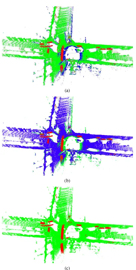
(a)
(b)
(c)
Figure 7. Moving object detection from a static laser scanner. (a) DST approach (R:moving, G:static, B:uncertain); (b) Probability approach (R:moving, G:uncertain, B:static); (c) ground truth of
moving object (R:moving)
balance between recall and precision, and has the highest F1
score.
3.2 Mobile Laser Scanning
As aforementioned, mobile laser scanning has been widely used for both environment mapping and autonomous navigation.
Mov-Method R% P% F1%
DST 83.0 57.3 67.8
Probability 74.1 66.4 70.1 Max-Distance 96.2 20.9 34.3 Nearest-point 60.1 70.1 64.7
Table 1. Accuracy assessment of moving object detection at point level from a static laser scanner.
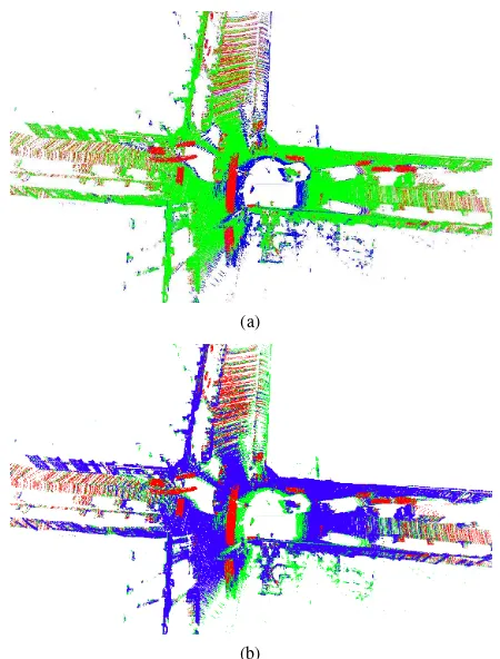
ing object detection from mobile laser scanning data is a funda-mental step in both fields. Occupancy-based methods will mani-fest their advantages as the laser scanner will cover different areas while moving forward, in which case the method needs to differ-entiate the real moving points from those that are out of the scan-ning scope. So the simple methods from the static laser scanscan-ning case,Max-DistanceandNearest-point, are no longer applicable. Only the two occupancy-based methods are evaluated. To keep the sensitivity to dynamics in the environment, the same settings as static laser scanning are used. Moving object detection results from a mobile laser scanner are demonstrated in Figure 8.
(a)
(b)
Figure 8. Moving object detection from a mobile laser scanner. (a) DST approach (R:moving, G:static, B:uncertain); (b)
Probability approach (R:moving, G:uncertain, B:static)
Moving point detection assessment without and with point nor-mals are listed in Table 2. DST approach shows a higher recall andF1 in both cases, whereas probability approach gives a
bet-ter precision. The detection with point normals shows significant improvements for both approaches. The results with normals are illustrated in Figure 9.
Method No normal With normal
R% P% F1% R% P% F1%
DST 81.9 53.9 65.0 80.1 84.2 82.5
Probability 71.1 57.4 63.6 66.0 92.1 76.9
Table 2. Accuracy assessment of moving object detection at point level from a mobile laser scanner.
(a)
(b)
(c)
Figure 9. Moving object detection with point normals using a mobile laser scanner. (a) DST approach (R:moving, G:static, B:uncertain); (b) Probability approach (R:moving, G:uncertain,
B:static); (c) ground truth of moving objects (R:moving)
4. DISCUSSION
Both DST and probability approaches define the occupancy of space first and fuse the occupancy information from multiple measurements, then efficiently assess the consistency between different scans. The probabilistic occupancy uses only one vari-able, the probability of being occupied, to model the space. Whereas the DST uses three variables to represent the three dif-ferent occupancy states,free,occupiedandunknown. The advan-tage is that it is able to distinguish the state of being half free half occupied (f = o = 0.5) and the state of being half occupied half unknown (o=u= 0.5). The former happens at the inter-face between free and occupied slightly before a point. The latter occurs behind the point when occupiedostarts to decrease and unknownuto increase. However, for the probability approach, the occupiedP(o) = 0.5in both cases, meaning there is no dif-ferentiation between the case of half free half occupied and the case of unknown. According to Section 2.2.3, the probability approach is actually the same as DST whenu= 0, meaning be-tween the laser center and the point the two methods will have the same results. Whenu∈ (0,1), the unknown evidence will contribute to the occupied value according the definition (Equa-tion 13). In practise, the implementa(Equa-tion details may cause dif-ference in terms of uncertainty modelling, occupancy interpola-tion and simplificainterpola-tion, such as log-odds transformainterpola-tion from the probabilistic occupancy.
The logit function is a simplification of the probability where multiplication is transferred to addition. Also to keep the sen-sitivity to the dynamic scene, the probability is truncated by the clamping thresholds. The the occupancy log-odds valueslf ree andlocchave to be carefully chosen. The advantage of proba-bilistic occupancy is the simplicity and computational efficiency. Note that in the static laser scanning case, the Nearest-point method can be considered as a naive way of interpreting the log-odds occupancy method. Each near point is counted as log-log-odds value 1, and the clamping threshold is the total number of nearest points. For the DST method, higher weight is given to the consis-tency evidence to reduce false alarms. However, there is not any mature simplification method such as logit function and clamp-ing. It is anticipated that a similar clamping strategy will also benefit in terms of simplicity and sensitivity to dynamics. Cur-rently the probability approach is preferred for efficient moving object detection.The DST is suitable for precise occupancy mod-elling and accurate moving object detection. More experiments are needed before drawing a decisive conclusion.
In both approaches, false detections are observed when the ground points are far from the laser center where the incidence angles are large. An effective solution is to model the occupancy along the normal direction instead of the ray direction around the point. Significant improvements are achieved after using the point normals. However, the normals have to be calculated be-forehand which may hinder real time or online moving object detection. Majority of these false detections are static ground points, they can either be filtered out first during environment mapping or simply be neglected during moving object tracking as these points will remain still over time. It is a question of the balance between accuracy and efficiency.
5. CONCLUSION
data using a real-time laser scanner. Two occupancy modelling approaches, DST and Probability, are introduced and compared theoretically. Detailed implementations are explained, from oc-cupancy definition, to evidence fusion, to the final consistency assessment. Similarities and differences are discussed. Both ap-proaches are applied to the two types of laser scanning data. Ex-perimental results are analysed and compared to other moving object detection methods where possible. Further improvement by involving the point normal is also proposed. DST provides a precise framework for occupancy modelling, whereas probability enables proper simplification and sensitivity improvement. Op-timised programming will be investigated in the future to further evaluate the computational efficiency of these two approaches.
REFERENCES
Aijazi, A. K., Checchin, P. and Trassoudaine, L., 2013. Detecting and updating changes in lidar point clouds for automatic 3d urban cartography. In:ISPRS Annals of Photogrammetry, Remote Sens-ing and Spatial Information Sciences, Vol. II-5/W2, pp. 7–12. Collins, T., 2011. Occupancy grid learning using contextual for-ward modelling. Journal of Intelligent & Robotic Systems 64(3-4), pp. 505–542.
Delafosse, M., Delahoche, L., Clerentin, A., Ricquebourg, V. and Jolly-Desodt, A. M., 2007. A dempster-shafer fusion architecture for the incremental mapping paradigm. In:International Confer-ence on Information Fusion, pp. 1–7.
Dezert, J., Moras, J. and Pannetier, B., 2015. Environment per-ception using grid occupancy estimation with belief functions. In: International Conference on Information Fusion, pp. 1070–1077. Girardeau-Montaut, D., Roux, M., Marc, R. and Thibault, G., 2005. Change detection on points cloud data acquired with a ground laser scanner. In: International Archives of the Pho-togrammetry, Remote Sensing and Spatial Information Sciences, Vol. 36, pp. 30–35.
Grabe, B., Ike, T. and Hoetter, M., 2009. Evidence based eval-uation method for grid-based environmental representation. In: International Conference on Information Fusion, pp. 1234–1240. Hebel, M., Arens, M. and Stilla, U., 2013. Change detection in urban areas by object-based analysis and on-the-fly comparison of multi-view als data. ISPRS Journal of Photogrammetry and Remote Sensing86, pp. 52–64.
Hornung, A., Wurm, K. M., Bennewitz, M., Stachniss, C. and Burgard, W., 2013. OctoMap: An efficient probabilistic 3D map-ping framework based on octrees.Autonomous Robots.
Kaestner, R., Maye, J., Pilat, Y. and Siegwart, R., 2012. Gen-erative object detection and tracking in 3d range data. In: IEEE International Conference on Robotics and Automation, pp. 3075– 3081.
Lindenbergh, R. and Pietrzyk, P., 2015. Change detection and deformation analysis using static and mobile laser scanning. Ap-plied Geomatics7(2), pp. 65–74.
Lindstr¨om, M. and Eklundh, J.-O., 2001. Detecting and tracking moving objects from a mobile platform using a laser range scan-ner. In:IEEE/RSJ International Conference on Intelligent Robots and Systems, Vol. 3, pp. 1364–1369.
Moosmann, F. and Stiller, C., 2011. Velodyne slam. In: IEEE Intelligent Vehicles Symposium, pp. 393–398.
Moosmann, F. and Stiller, C., 2013. Joint self-localization and tracking of generic objects in 3d range data. In: IEEE Interna-tional Conference on Robotics and Automation, pp. 1146–1152. Moras, J., Dezert, J. and Pannetier, B., 2015. Grid occupancy estimation for environment perception based on belief functions and PCR6. In:SPIE Defense+ Security, p. 94740P.
Murphy, R., 1998. Dempster-shafer theory for sensor fusion in autonomous mobile robots. IEEE Transactions on Robotics and Automation14(2), pp. 197–206.
Paparoditis, N., Papelard, J., Cannelle, B., Devaux, A., Soheil-ian, B., David, N. and Houzay, E., 2012. Stereopolis ii: A multi-purpose and multi-sensor 3d mobile mapping system for street visualisation and 3d metrology. Revue Franc¸aise de Pho-togramm´etrie et de T´el´ed´etection200, pp. 69–79.
Payeur, P., 2003. Fuzzy logic inference for occupancy state mod-eling and data fusion. In: IEEE International Symposium on Computational Intelligence for Measurement Systems and Appli-cations, pp. 175–180.
Shafer, G., 1992. The dempster-shafer theory. Encyclopedia of artificial intelligencepp. 330–331.
Thrun, S., 2002. Learning occupancy grids with forward sensor models.Autonomous Robots15, pp. 111–127.
Vallet, B., Xiao, W. and Br´edif, M., 2015. Extracting mobile ob-jects in images using a velodyne lidar point cloud. In: ISPRS Annals of the Photogrammetry, Remote Sensing and Spatial In-formation Sciences, Vol. 1, pp. 247–253.
Vu, T.-D., Burlet, J. and Aycard, O., 2011. Grid-based localiza-tion and local mapping with moving object deteclocaliza-tion and track-ing.Information Fusion12(1), pp. 58–69.
Wolf, D. and Sukhatme, G. S., 2004. Online simultaneous local-ization and mapping in dynamic environments. In: IEEE Inter-national Conference on Robotics and Automation (ICRA), Vol. 2, pp. 1301–1307.
Xiao, W., Vallet, B., Br´edif, M. and Paparoditis, N., 2015. Street environment change detection from mobile laser scanning point clouds. ISPRS Journal of Photogrammetry and Remote Sensing 107, pp. 38–49.
Xiao, W., Vallet, B., Schindler, K. and Paparoditis, N., 2016. Si-multaneous detection and tracking of pedestrian from panoramic laser scanning data. In: ISPRS Annals of Photogrammetry, Remote Sensing and Spatial Information Sciences, Vol. III-3, pp. 295–302.
Xu, S., Vosselman, G. and Oude Elberink, S., 2013. Detection and classification of changes in buildings from airborne laser scanning data. In: ISPRS Annals of Photogrammetry, Remote Sensing and Spatial Information Sciences, Vol. II-5/W2, pp. 343– 348.
Yager, R. R. and Liu, L., 2008. Classic works of the Dempster-Shafer theory of belief functions. Vol. 219, Springer.
Yguel, M., Aycard, O. and Laugier, C., 2007. Update policy of dense maps: Efficient algorithms and sparse representation. In: International Conference on Field and Service Robotics, Vol. 42, pp. 23–33.