IDC Engineering Pocket Guide
PO Box 1093, West Perth WA 6872 Tel: (08) 9321 1702 Fax: (08) 9321 2891
Suite 402, 814 Richards Street, Vancouver BC V6B 3A7
Tel: (604) 244 9221 Fax: (604) 682 3139 Toll Free Tel: 1800 324 4244
Toll Free Fax: 1800 434 4045
India
PO Box 8069, Shankill, Co Dublin Tel: (01) 473 3190 Fax: (01) 473 3191
Malaysia
26 Jalan Kota Raja E27/E, Hicom Town Center, Seksyen 27, 40400 Shah Alam, Selangor
Tel: (03) 5192 3800 Fax: (03) 5192 3801
New Zealand
Parkview Towers, 28 Davies Avenue, Manukau City
PO Box 76-142, Manukau City Tel: (09) 263 4759 Fax: (09) 262 2304
Poland
ul. Krakowska 50, 30-083 Balice, Krakow Tel: +48 12 6304 746 Fax: +48 6304 750
Singapore
100 Eu Tong Sen Street, #04-11 Pearl's Centre, Singapore 059812
Tel: (65) 6224 6298 Fax: (65) 6224 7922
South Africa
68 Pretorius Street, President Park, Midrand PO Box 389, Halfway House 1685 Tel: (011) 805 3904 Fax: (011) 312 2150 Toll Free Tel: 0800 114 160
United Arab Emirates
M1 Floor, Khalifa Street, Al Za’abi Building, Abu Dhabi, UAE Tel: +971 2 676 4470 Fax: +971 2 676 4490
United Kingdom
Suite 18, Fitzroy House, Lynwood Drive, Worcester Park, Surrey KT4 7AT Tel: (020) 8335 4014 Fax: (020) 8335 4120
United States
7101 Highway 71 West #200, Austin TX 78735 Tel: (512) 288 8525 Fax: (512) 288 8521 Toll Free Tel: 1800 324 4244
_________________________________
Pocket Guide on
Industrial Automation
For Engineers and Technicians
Rev 1.04
Edited by
Srinivas Medida
Chapter 1.
Introduction...6
Chapter 2.
I&C Drawings and Documentation ...7
2.1.
Introduction to Plant Design ...7
2.2. Process
diagrams...7
2.3. Instrumentation
documentation ...11
2.4. Electrical
documentation ...15
Chapter 3.
Process control ...18
3.1.
Basic Control Concepts...18
3.2.
Principles of Control Systems...19
3.3.
Control modes in closed loop control ...23
3.4.
Tuning of Closed Loop Control...24
3.5. Cascade
Control ...27
3.6.
Initialization of a cascade system ...27
3.7.
Feed forward Control...27
3.8.
Manual feedforward control ...28
3.9.
Automatic feedforward control...28
3.10.
Time matching as feedforward control ...28
3.11.
Overcoming Process dead time...29
3.12.
First term explanation(disturbance free PV)...30
3.13.
Second term explanation(predicted PV) ...30
Chapter 4.
Advanced Process Control...31
4.1. Introduction...31
4.2.
Overview of Advance Control Methods ...31
4.3.
Internal Model Control ...33
Chapter 5.
Industrial Data Communications and Wireless...36
5.1. Introduction...36
5.2.
Open Systems Interconnection (OSI) model ...36
5.3.
RS-232 interface standard...37
5.4. Fiber
Optics...39
5.5. Modbus ...40
5.6.
Data Highway Plus /DH485...44
5.7. HART...45
5.14. Wireless
Fundamentals ...52
5.15. Radio/microwave
communications...53
5.16. Installation
&
Troubleshooting ...53
5.17.
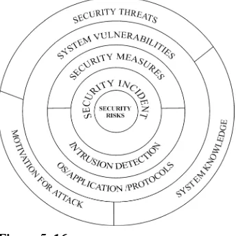
Industrial network security ...59
5.18.
Network threats, vulnerabilities and risks...60
5.19.
An approach to network security planning ...62
5.21. Authentication,
Authorization, Accounting & encryption...63
5.22. Intrusion
detection
systems...65
5.23. VLANs...65
5.24.
VPNs and their security ...66
5.25.
Wireless networks and their security issues ...67
Chapter 6.
HAZOPs Hazard Operations ...69
6.1. Introduction...69
6.2. HAZOP
Workshop ...70
Chapter 7.
Safety Instrumentation and Machinery...72
7.1. Introduction...72
7.2.
Introduction to IEC 61511 and the safety lifecycle ...80
7.3.
SIS configurations for safety and availability targets...84
7.4.
Selection of sensors and actuators for safety duties ...87
7.5.
Selection of safety controllers...92
7.6.
System integration and application software ...92
7.7. Programming
tools...93
7.8. Machinery
safety...94
7.9.
Guide to Regulations and Standards...95
Chapter 8.
Hazardous Areas and Intrinsic Safety...98
8.1. Introduction...98
8.2. Zonal
Classification ...100
8.3. Area
classification...101
8.4.
Methods of explosion protection ...103
8.5. Flameproof
concept
Ex
d...104
8.6. Intrinsic
safety...105
8.7. Increased
safety...107
8.8. Certification
(components) ...108
8.9.
Principles of testing ...108
8.10.
Non Sparking concept...109
8.11.
Concept Ex p...110
8.12.
Other protection concepts ...112
8.13.
Earthing & Bonding...114
8.14.
Standards and codes of practice...115
8.15.
Fault finding and repairs ...115
Chapter 9.
SCADA...118
9.1.
Introduction and Brief History of SCADA...118
9.2.
SCADA Systems Software ...121
9.3. Distributed
control system (DCS)...129
9.4.
Introduction to the PLC ...132
9.5.
Considerations and benefits of SCADA system ...134
9.6.
An alarm system ...135
Chapter 10.
Project Management of I&C Projects...140
10.1.
Fundamentals of project management ...140
10.2. Time
management...142
10.3. Cost
Management ...143
10.5.
Management of project team ...144
10.6. Risk
Management ...145
10.7. Contract
law ...146
Chapter 11.
Latest Instrumentation and Valve Developments ...150
11.1.
Basic Measurement performance terms and Specifications ...150
11.2.
Advanced Measurement Performance terms and Specifications...151
11.3. Pressure
Measurement ...152
11.4. Level
Measurement...156
11.5. Temperature
Measurement ...158
11.6. Thermocouples...158
11.7. Resistance
Temperature Detectors (RTD’s) ...159
11.8. Thermistors ...159
11.9. Infrared
Pyrometers ...160
11.10. Acoustic
Pyrometers ...160
11.11. Flow
Measurement...160
11.12. Differential
Pressure
Flowmeters ...162
11.13. Magnetic
Flowmeters...164
11.14. Control
Valves ...166
Chapter 12.
Forecasts and Predictions...168
12.1.
Main Technology Trends...168
12.2.
The China Challenge...169
Preface
Industrial Automation is a discipline that includes knowledge and expertise from various branches of engineering including electrical, electronics, chemical, mechanical, communications and more recently computer and software engineering. Automation & Control by its very nature demands a cross fertilization of these faculties.
Industrial Automation Engineers have always drawn new technologies and implemented original or enhanced versions to meet their requirements. As the range of technology diversifies the demand on the innovative ability of these Engineers has increased.
IDC Technologies has been in the business of bringing together the domain gurus and the practicing engineers under an umbrella called training. The sum of the knowledge that IDC Technologies has acquired over many years has now given it an opportunity to compile this comprehensive hand book for the reference of every automation engineer.
The breadth and depth of Industrial Automation is enormous and justice cannot be expected from a book of a few hundred pages. This book comprises over 1200 pages of useful, hard hitting information from the trenches on industrial automation. This book delivers a critical blend of knowledge and skills, covering technology in control and instrumentation, industry analysis and forecasts, leadership and management - everything that is relevant to a modern control and instrumentation engineer. Good management, financial and business skills are also provided in these chapters. These highly practical materials provide you with solid skills in this often neglected area for control and instrumentation engineers.
This book was originally written for UK and other European users and contains many references to the products and standards in those countries. We have made an effort to include IEEE/ANSI/NEMA references wherever possible. The general protection approach and theoretical principles are however universally applicable.
The terms ‘earth’ as well as ‘ground’ have both been in general use to describe the
common power/signal reference point interchangeably around the world in the Electro-technical terminology. While the USA and other North American
countries favor the use of the term ‘ground’, European countries including the UK
and many other Eastern countries prefer the term ‘earth’. In this book, we chose to
adopt the term ‘ground’ to denote the common electrical reference point. Our
sincere apologies to those readers who would have preferred the use of the term ‘earth’.
Chapter 1. Introduction
Society in its daily endeavours has become so dependent on automation that it is difficult to imagine life without automation engineering. In addition to the industrial production with which it is popularly associated, it now covers a number of unexpected areas. Trade, environmental protection engineering, traffic engineering, agriculture, building engineering, and medical engineering are but some of the areas where automation is playing a prominent role. Automation engineering is a cross sectional discipline that requires proportional knowledge in hardware and software development and their applications. In the past, automation engineering was mainly understood as control engineering dealing with a number of electrical and electronic components. This picture has changed since computers and software have made their way into every component and element of communications and automation.
Industrial automation engineers carry a lot of responsibility in their profession. No other domain demands so much quality from so many perspectives of the function, yet with significant restrictions on the budget. The project managers of industrial automation projects have significant resource constraint, considering the ever changing demands of its management, trying to adopt the rapid acceleration of the technological changes and simultaneously trying to maintain the reliability and unbreakable security of the plant and its instruments.
Chapter 2. I&C Drawings and
Documentation
2.1.
Introduction to Plant Design
Plant design (process plant design, power plant design, etc.) refers to the automation technologies, work practices and business rules supporting the design and engineering of process and power plants. Such plants can be built for chemical, petroleum, utility, shipbuilding, and other facilities. Plant design is used to designate a general market area by the many vendors offering technologies to support plant design work.
2.2. Process
diagrams
The ‘process’ is an idea or concept that is developed to a certain level in order to determine the feasibility of the project. ‘Feasibility’ study is the name given to a small design project that is conducted to determine the scope and cost of implementing the project from concept to operation.
To keep things simple, for example, design an imaginary coffee bottling plant to produce bottled coffee for distribution. Start by creating a basic flow diagram that illustrates the objective for the proposed plant; this diagram is called a “Process Block Diagram”.
2.2.1. Process block diagram
The block diagram shown in Figure 2. 1 is where it all starts. It is here that the basic components are looked at and the basic requirements determined. This is a diagram of the concept, giving a very broad view of the process.
Figure 2. 1
Basic flow diagram of Coffee bottling plant
2.2.2. Process flow diagram or piping flow diagram (PFD)
The PFD is where we start to define the process by adding equipment and the piping that joins the various items of equipment together. The idea behind the PFD is to show the entire process (the big picture) on as few drawing sheets as possible, as this document is used to develop the process plant and therefore the process engineer wants to see as much of the process as possible. This document is used to determine details like the tank sizes and pipe sizes.
Those familiar with mimic panels and SCADA flow screens will notice that these resemble the PFD more than the piping and instrumentation diagram (P&ID) with the addition of the instruments, but not the instrument function.
Mass balance: In its most simple form, what goes in must come out. The totals at the end of the process must equal the totals fed into the system.
2.2.3. Process description
The process description details the function / purpose of each item of equipment in the plant. This description should contain the following information:
• Installation operation – The installation produces bottled coffee
• Operating principles – Each part of the process is described
• Water supply – Filtered water at ambient temperature is supplied to
the water holding tank, the capacity of the tank should be sufficient for all recipes
• Coffee supply – Due to the viscosity of the coffee syrup, the syrup is
fed from a pressurized vessel to the autoclave, this line should be cleaned frequently with warm water. There will be batches of caffeinated and decaffeinated coffee, the coffee tanks and pipelines must be thoroughly cleaned between batches
• Milk supply – There will be an option for low fat or full cream milk,
the milk supply should be sufficient for three days operation and should be kept as close to freezing as possible to ensure longevity of the milk
• Sugar supply – Sugar will be supplied in a syrup form, we will offer
the coffee with no sugar, 1 teaspoon (5 ml of syrup) or two teaspoons (10 ml of syrup). Syrup lines must be cleaned on a regular basis
• Circuit draining/make-up – How to start-up or shutdown the facility,
• Liquid characteristics – A detailed description on analysis of each liquid type in the system. Includes specific gravity, viscosity, temperature, pressure, composition etc.
• Specific operating conditions linked to the process – The installation
operates 24 hours a day, 365 days a year. As the installation deals with foodstuff, all piping and vessels are to be manufactured from stainless steel
• Specific maintenance conditions linked to the process – Hygiene
levels to be observed
• Specific safety conditions linked to the process – Hygiene,
contamination of product
• Performance requirements – This section describes the amount of
product the plant must be able to produce in a given time frame.
PFD now starts to look something like the Figure 2. 2 shown below.
Figure 2. 2
Process flow diagram
2.2.4. Piping and Instrumentation Diagram (P&ID)
The Piping & Instrumentation Diagram, which may also be referred to as the Process & Instrumentation Diagram, gives a graphical representation of the process including hardware (Piping, Equipment) and software (Control systems); this information is used for the design construction and operation of the facility.
The PFD defines “The flow of the process” The PFD covers batching, quantities, output, and composition.
The P&ID ties together the system description, the flow diagram, the electrical control schematic, and the control logic diagram. It accomplishes this by showing all of the piping, equipment, principal instruments, instrument loops, and control interlocks. The P&ID contains a minimum of text in the form of notes (the system description minimizes the need for text on the P&ID).
The typical plant operation’s environment uses the P&ID as the principal document to locate information about the facility, whether this is physical data about an object, or information, such as financial, regulatory compliance, safety, HAZOP information, etc.
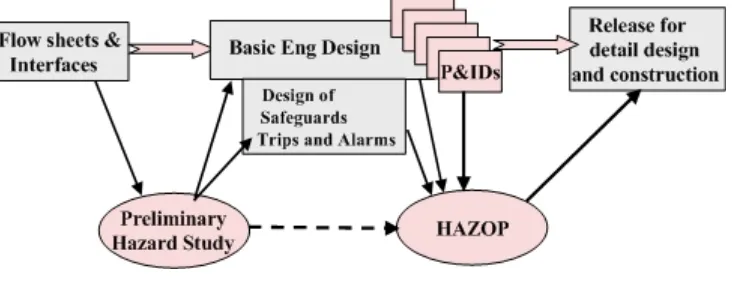
The P&ID defines “The control of the flow of the process” where the PFD is the main circuit; the P&ID is the control circuit. Once thoroughly conversant with the PFD & Process description, the engineers from the relevant disciplines (piping, electrical & control systems) attend a number of HAZOP sessions to develop the P&ID.
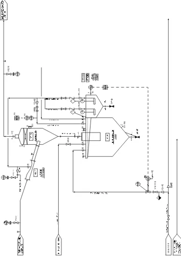
2.2.5. P&ID standards
Before development of the P&ID can begin, a thorough set of standards is required. These standards must define the format of each component of the P&ID. The following should be shown on the P&ID:
• Mechanical Equipment
• Equipment Numbering
• Presentation on the P&ID
• Valves
• Hand valves
• Control valves
• Piping
• Pipe numbering
• Nozzles & Flanges
• Equipment & instrument numbering systems
Figure 2. 3 Completed P&ID
2.3.
Instrumentation documentation
The best way to understand the purpose and function of each document is to look at the complete project flow from design through to commissioning.
• Design
• Design criteria, standards, specifications, vendor lists
• Construction
• Quantity surveying, disputes, installation contractor, price per meter,
per installation
• Operations
• Maintenance commissioning
2.3.1. Instrument list
This is a list of all the instruments on the plant, in the ‘List’ format. All the instruments of the same type (tag) are listed together; for example, all the pressure transmitters ‘PT’ are grouped together.
Instrument index lists Associated documentation such as loop drawing
number, datasheets, installation details and P&ID.
Loop List The same information as the instrument list but
ordered by loop number instead of tag number. This sort of order will group all elements of the same loop number together.
Function Gives a list of all the instrumentation on the plant and
may include ‘virtual’ instruments such as controllers in a DCS or PLC.
Tag No The instrument tag number as defined by the
specification.
Description Description of the instrument as denoted by the tag
number.
Service Description A description of the process related parameter.
Functional Description The role of the device.
Manufacturer Details of the manufacturer of the device.
Model Details of the model type and number.
Table 2. 1 Instrument list
2.3.2. Instrument location plans
The instrument location drawing is used to indicate an approximate location of the instruments and junction boxes. This drawing is then used to determine the cable lengths from the instrument to the junction box or control room. This drawing is also used to give the installation contractor an idea as to where the instrument should be installed.
2.3.3. Cable racking layout
Figure 2. 4 Cable racking layout
2.3.4. Cable routing layout
Prior to the advent of 3D CAD packages, the routing layout used a single line to indicate the rack direction as well as routing and sizes and was known as a ‘Racking & Routing layout’.
Figure 2. 5 Cable routing layout
2.3.5. Block diagrams – signal, cable and power block diagrams
Figure 2. 6 Block diagram
Field connections / Wiring diagrams
Function
To instruct the wireman on how to wire the field cables at
the junction box.
Used by
The installation contractor. When the cable is installed on
the cable rack, it is left lying loose at both the instrument
and junction box ends. The installation contractor stands at
the junction box and strips each cable and wires it into the
box according to the drawing.
Table 2. 2
Field connections / Wiring diagrams
Power distribution diagram
Function
There are various methods of supplying power to field
instruments; the various formats of the power distribution
diagrams show these different wiring systems.
Used by
Various people depending on the wiring philosophy, such
as the panel wireman, field wiring contractor.
Table 2. 3
Power distribution diagram
Earthing diagram
Function
Used to indicate how the earthing should be done. Although
this is often undertaken by the electrical discipline, there are
occasions when the instrument designer may or must
generate his own scheme – Eg. for earthing of zener barriers
in a hazardous area environment.
Used by
Earthing contractor for the installation of the earthing. This
drawing should also be kept for future modifications and
reference.
Table 2. 4 Earthing diagram
Loop diagrams
Function
A diagram that comprehensively details the wiring of the
loop, showing every connection from field to instrument or
I/O point of a DCS/PLC.
Used by
Maintenance staff during the operation of the plant and by
commissioning staff at start up.
Table 2. 5 Loop diagrams
2.4. Electrical
documentation
2.4.1. The Load List
The load list is used to total the power supply requirements for each device per plant area or process. Load lists are made for each voltage level on the plant. The sample table shown below is a typical layout of a load list.
Device Voltage Amps Watts VA Total Feeder
400-PMP-01 380 400-TAD-01
Table 2. 6 Sample
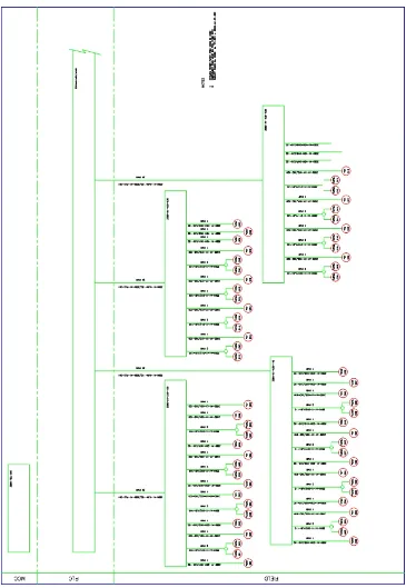
2.4.2. The Single Line Diagram
The single line diagram (sometimes called the one line diagram) uses single lines and standard symbols to show electrical cables, bus bars and component parts of a circuit or system of circuits. The single line diagram shows the overall strategy for system operation. Duplication of a 3-wire system is reduced by showing single devices on a single wire. These single line diagrams may be used in the monitoring and control systems like SCADA applications for the operation.
2.4.3. The schematic diagram (main and circuit)
Schematic diagram shows both the main circuit and the control circuit in far greater detail; here all three lines of a 3-phase system are shown. The schematic shows the detailed layout of the control circuit for maintenance and faultfinding purposes rather than the overall picture presented by the single line diagram.
A schematic diagram shows the following main features:
• Main circuits
• Control, signal and monitoring circuits
• Equipment identification symbols with component parts and
connections
• Equipment and terminal numbering
• Cross references – indicating where on the diagram or sequential
sheet, the related parts of the equipment can be found.
2.4.4. Plant layout drawings
The plant layout drawing gives a physical plant layout, where equipment is drawn to resemble the plant item it represents.
2.4.5. Racking and Routing
2.4.6. Installation Details
The installation detail shows the layout of the equipment and gives an itemized list of all the equipment on the drawing as well as notes on the installation.
2.4.7. Panel Layout
The panel layout drawing gives the dimensions of the panel, the layout of the equipment in the panel, an itemized list of all the equipment used as well as quantities. The notes detail various items like specification references (paint, powder coating) and general notes.
2.4.8. Other electrical documents
Cable schedule: This is used mainly for installation purposes. It gives a source and destination for each cable and specifies the type of cable.
Point to point schedule: This facilitates wiring installation by showing termination points at each end of every wire.
Hazardous area drawings: A plant location drawing (in both plan and elevation) which shows, by means of overlays, plant area classifications (by zone and gas group) for potential leak hazards throughout a plant.
Ladder Logic Schematics: These are detailed schematics of a ladder structure
Chapter 3. Process control
3.1.
Basic Control Concepts
Most basic process control systems consist of a control loop as shown in Figure 3. 1. This has four main components which are:
• A measurement of the state or condition of a process
• A controller calculating an action based on this measured value
against a pre-set or desired value (set point)
• An output signal resulting from the controller calculation which is
used to manipulate the process action through some form of actuator
• The process itself reacting to this signal, and changing its state or
condition.
Figure 3. 1
Block diagram showing the elements of a process control loop
Two of the most important signals used in process control are called
• Process Variable or PV
• Manipulated Variable or MV
display so that the operator can use the reading to adjust the process through manual control and supervision.
The variable to be manipulated, in order to have control over the PV, is called the Manipulated Variable. If we control a particular flow for instance, we manipulate a valve to control the flow. Here, the valve position is called the Manipulated Variable and the measured flow becomes the Process Variable.
3.2.
Principles of Control Systems
To perform an effective job of controlling a process, we need to know how the control input we are proposing to use will affect the output of the process. If we change the input conditions we need to know the following:
• Will the output rise or fall?
• How much response will we get?
• How long will it take for the output to change? .
• What will be the response curve or trajectory of the response?
The answers to these questions are best obtained by creating a mathematical model of the relationship between the chosen input and the output of the process in question. Process control designers use a very useful technique of block diagram modeling to assist in the representation of the process and its control system. The following section introduces the principles that should apply to most practical control loop situations.
The process plant is represented by an input/output block as shown in Figure 3. 2
Figure 3. 2
Basic block diagram for the process being controlled
In Figure 3. 2, we see a controller signal that will operate on an input to the process, known as the ‘manipulated variable’. We try to drive the output of the process to a particular value or set point by changing the input. The output may also be affected by other conditions in the process or by external actions such as changes in supply pressures or in the quality of materials being used in the process. These are all regarded as ‘disturbance inputs’ and our control action will need to overcome their influences as well as possible.
example, if we want to keep the level of water in a tank at a constant height while others are drawing off from it, we will manipulate the input flow to keep the level steady.
The value of a process model is that it provides a means of showing the way the output will respond to the input actions. This is done by having a mathematical model based on the physical and chemical laws affecting the process.
For example in Figure 3. 3, an open tank with cross sectional area A is
supplied with an inflow of water Q1 that can be controlled or manipulated. The
outflow from the tank passes through a valve with a resistance R to the output
flow Q2. The level of water or pressure head in the tank is denoted as H. We know
that Q2 will increase as H increases and when Q2 equals Q1 the level will become
steady.
The block diagram of this process is shown in Figure 3. 4
Figure 3. 3
Example of a water tank with controlled inflow
Figure 3. 4
3.2.1. Stability
A closed loop control system is stable if there is no continuous oscillation. A noisy and disturbed signal may show up as a varying trend; but it should never be confused with loop instability. The criteria for stability are these two conditions:
• The Loop Gain (KLOOP) for the critical frequency <1;
• Loop Phase Shift for the critical frequency < 180°.
3.2.2. Loop gain for critical frequency
Consider the situation where the total gain of the loop for a signal with that frequency has a total loop phase shift of 180°. A signal with this frequency is decaying in magnitude, if the gain for this signal is below 1. The other two alternatives are:
• Continuous oscillations which remain steady (Loop Gain = 1);
• Continuous oscillations which are increasing, or getting worse
(Loop Gain > 1).
3.2.3. Loop phase shift for critical frequency
Consider the situation where the total phase shift for a signal with that frequency has a total loop gain of 1. A signal with this phase shift of 180° will generate oscillations if the loop gain is greater than 1. Increasing the Gain or Phase Shift destabilizes a closed loop, but makes it more responsive or sensitive.
Decreasing the Gain or Phase Shift stabilizes a closed loop at the expense of making it more sluggish.
The gain of the loop (KLOOP) determines the OFFSET value of the controller; and
offset varies with Set point changes.
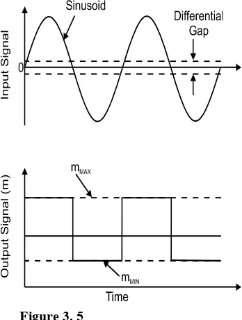
3.2.4. Control Modes
Figure 3. 5
Response of a two positional controller to a sinusoidal input
Modulating control: If the output of a controller can move through a range of values, this is modulating control.
Modulation Control takes place within a defined operating range only. That is, it must have upper and lower limits. Modulating control is a smoother form of control than step control. It can be used in both open loop and closed loop control systems.
Open loop control: Open loop control is thus called because the control action (Controller Output Signal OP) is not a function of the PV (Process Variable) or load changes. The open loop control does not self-correct, when these PV’s drift.
Feed forward control: Feed forward control is a form of control based on anticipating the correct manipulated variables required to deliver the required output variable. It is seen as a form of open loop control as the PV is not used directly in the control action.
Figure 3. 6
The feedback control loop
The idea of closed loop control is to measure the PV (Process Variable); compare this with the SP (Set Point), which is the desired, or target value; and determine a control action which results in a change of the OP (Output) value of an automatic controller.
In most cases, the ERROR (ERR) term is used to calculate the OP value.
ERR = PV - SP
If ERR = SP - PV has to be used, the controller has to be set for REVERSE control action.
3.3.
Control modes in closed loop control
Most Closed loop Controllers are capable of controlling with three control modes which can be used separately or together
• Proportional Control (P)
• Integral, or Reset Control (I)
• Derivative, or Rate Control (D)
3.3.1. Proportional control(P)
This is the principal means of control. The automatic controller needs to correct the controllers OP, with an action proportional to ERR. The correction starts from an OP value at the beginning of automatic control action.
Proportional error and manual value: This is called as starting value manual. In the past, this has been referred to as "manual reset". In order to have an automatic correction made, that means correcting from the manual starting term, we always need a value of ERR. Without an ERR value there is no correction and go back to the value of manual.
3.3.2. Integral control(I)
Integral action is used to control towards no OFFSET in the output signal. This means that it controls towards no error (ERR = 0). Integral control is normally used to assist proportional control. The combination of both is called as PI-control.
Formula for I-Control:
Tint is the Integral Time Constant.
3.3.3. Derivative control (D)
The only purpose of derivative control is to add stability to a closed loop control system. The magnitude of derivative control (D-Control) is proportional to the rate of change (or speed) of the PV.
Since the rate of change of noise can be large, using D-Control as a means of enhancing the stability of a control loop is done at the expense of amplifying noise. As D-Control on its own has no purpose, it is always used in combination with P-Control or PI-Control. This results in a PD-Control or Control. PID-Control is mostly used if D-PID-Control is required.
Formula for D-Control:
Tder is the Derivative Time Constant.
3.4.
Tuning of Closed Loop Control
There are often many and sometimes contradictory objectives, when tuning a controller in a closed loop control system. The following list contains the most important objectives for tuning of a controller:
Figure 3. 7
Integral on error
Minimization of the integral of the error squared: As shown in Figure 3. 8, it is possible to have a small area of error but an unacceptable deviation of PV from SP for a start time. In such cases, special weight must be given to the magnitude of the deviation of PV from SP. Since the weight given is proportional to the magnitude of the deviation, the weight is multiplied by the error. This gives error squared (error squared = error * weight). Many modern controllers with automatic and continuous tuning work on this basis.
Figure 3. 8
Integral on error square
Fast control: In most cases, fast control is a principle requirement from an operational point of view. However, this is principally achieved by operating the controller with a high gain. This quite often results in instability, or prolonged settling times from the effects of process disturbances.
Minimum wear and tear of controlled equipment: A valve or servo system for instance should not be moved unnecessarily frequently, fast or into extreme positions. In particular, the effects of noise, excessive process disturbances and unrealistically fast controls have to be considered here.
Minimizing the effect of known disturbances: If we can measure disturbances, we may have a chance to control them before their effects become apparent.
3.4.1. Continuous cycling method (Ziegler Nichols)
This method of tuning requires determining the critical value of controller gain
(KC) that will produce a continuous oscillation of a control loop. This will occur
when the total loop gain (KLOOP) is equal to one. The controller gain value (KC)
then becomes known as the ultimate gain (KU).
If we consider a basic liquid flow control loop utilizing:
• A venturi flow meter with a 4-20 mA output feeding into…
• a PID controller which in turn has a 4-20 mA output that controls...
• a valve actuator that in turn varies the flow rate of…
• the process.
When the product of the gains of all four of these component parts equals one, the system will become unstable when a process disturbance occurs (a set-point change). It will oscillate at its natural frequency which is determined by the process lag and response time, and caused by the loop gain becoming one.
Then measure the frequency of oscillation (the period of one cycle of oscillation), this being the ultimate period PU.
In addition, the final value of KC is the critical gain of the controller (KU). This
gain value, when multiplied with the unknown process Gain(s), will give a Loop Gain, KLOOP, of 1.
3.4.2. The stages of obtaining closed loop tuning (continuous cycling method)
• Put Controller in P-Control Only
• Select the P-Control to ERR = (SP - PV)
• Put the Controller into Automatic Mode
• Make a Step Change to the Set point
• Take action based on the Observation
• Conclude the Tuning Procedure.
3.4.3. Damped cycling tuning method
This method is a variation of the continuous cycling method. It is used whenever continuous cycling imposes a danger to the process, but a damped oscillation of some extent is acceptable.
The steps of closed loop tuning (damped cycling method) are as follows:
• Put the Controller into P-Control Only
• Select the P-Control to ERR = (SP - PV)
• Put the Controller in Automatic Mode
• Make a Step Change to the Set point
3.5. Cascade
Control
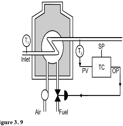
If the OP of the temperature controller TC drives the SP of this newly added fuel flow controller FC, then there is a situation that the OP of the temperature controller TC then drives the true flow and not just a valve position.
Fuel flow pressure would practically have no effect on the outlet temperature. This concept is called ‘cascade control’. The principle is shown in Figure 3. 9.
Figure 3. 9
Single loop temperature control
3.5.1. The concept of process variable or PV-tracking
PV-Tracking is active if the secondary (FC) controller is in manual mode. Controllers can be set up to make use of PV-Tracking or not.
The concept is that an operator sets the OP value of the fuel controller manually until they find an appropriate value for the process.
3.6.
Initialization of a cascade system
Initialization is actually a kind of manual mode where the operator does not drive the OP value of the primary controller. (temperature controller, TC, in this case.) Instead, fuel controller FC supplies its set point (SP) value, back up the cascade chain to the OP of the controller that will be driving it (the FC’s SP) when the system is in automatic mode. If selected, PV-Tracking can take place in the primary controller as it would occur in normal manual mode.
3.7.
Feed forward Control
If, within a process control’s feedback system, large and random changes to either the PV or Lag time of the process occur, the feedback action becomes very ineffective in trying to correct these excessive variances.
The result of this is that the accuracy and standard of the process becomes unacceptable. Feedforward control is used to detect and correct these disturbances before they have a chance to enter and upset the closed or feedback loop characteristics.
Feedforward Control has
• Manual feedforward control
• Automatic feedforward control
3.8.
Manual feedforward control
Here, as a disturbance enters the process, it is detected and measured by the process operator. Based on his knowledge of the process, the operator then changes the manipulated variable by an amount that will minimize the effect of the measured disturbance on the system.
This form of feedforward control relies heavily on the operator and his knowledge of the operation of the process. However, if the operator makes a mistake or is unable to anticipate a disturbance, then the controlled variable will deviate from its desired value and, if feedforward is the only control, an uncorrected error will exist.
3.9.
Automatic feedforward control
Disturbances that are about to enter a process are detected and measured. Feedforward controllers then change the value of their manipulated variables (outputs) based on these measurements as compared with their individual set-point values.
Feedforward controllers must be capable of making a whole range of calculations, from simpe on-off action to very sophisticated equations. These calculations have to take into account all the exact effects that the disturbances will have on controlled variables.
Pure feedforward control is rarely encountered; it is more common to find it embedded within a feedback loop where it assists the feedback controller function by minimizing the impact of excessive process disturbances.
3.10.
Time matching as feedforward control
Time taken for a process to react in one direction (heating) is different to the time taken for the process to return to its original state (cooling). If the reaction curve (dynamic behavior of reaction) of the process disturbance is not equal to the control action, it has to be made equal.
3.10.1. Process dead time
Overcoming the dead time in a feedback control loop can present one of the most difficult problems to the designer of a control system. This is especially true if the dead time is greater than 20% of the total time taken for the PV to settle to its new value after a change to the SP value of a system.
If the time from a change in the manipulated variable (controller output) and a detected change in the PV occurs, any attempt to manipulate the process variable before the dead time has elapsed will inevitably cause unstable operation of the control loop. Figure 3. 10 illustrates various dead times and their relationship to the PV reaction time.
Figure 3. 10
Reaction curves showing short, medium and long dead times
3.11.
Overcoming Process dead time
Solving these problems depends to a great extent on the operating requirement(s) of the process. The easiest solution is to “de-tune” the controller to a slower response rate. The controller will then not overcompensate unless the dead time is excessively long.
The integrator (I mode) of the controller is very sensitive to “dead time” as during this period of inactivity of the PV (an ERR term is present) the integrator is busy “ramping” the output value.
Ziegler and Nichols determined the best way to “de-tune” a controller, to handle a
dead time of D minutes, is to reduce the integral time constant TINT by a factor of
D2 and the Proportional constant by a factor of D.
The derivative time constant TDER is unaffected by dead time as it only occurs after
the PV starts to move.
3.12.
First term explanation(disturbance free PV)
The first term is an estimate of what the PV would be like in the absence of any process disturbances. It is produced by running the controller output through a model that is designed to accurately represent the behavior of the process without taking any load disturbances into account. This model consists of two elements connected in series.
• The first represents all of the process behavior not attributable to
dead time. This is usually calculated as an ordinary differential or difference equation that includes estimates of all the process gains and time constants.
• The second represents nothing but the dead time and consists simply
of a time delay, what goes in, comes out later, unchanged.
3.13.
Second term explanation(predicted PV)
The second term introduced into the feedback path is an estimate of what the PV would look like in the absence of both disturbances and dead time. It is generated by running the controller output through the first element of the model (gains and TC’s) but not through the time delay element.
It thus predicts what the disturbance-free PV will be like once the dead time has elapsed.
Figure 3. 11
The smith predictor in use
If it is successful in doing so and the process model accurately emulates the process itself, then the controller will simultaneously drive the actual PV toward the SP value, irrespective of SP changes or load disturbances.
Chapter 4. Advanced Process
Control
4.1. Introduction
Advanced process control (APC) is a broad term within the control theory. It is composed of different kinds of process control tools, for example, model predictive control (MPC), statistical process control (SPC), Run2Run (R2R), fault detection and classification (FDC), sensor control and feedback systems. APC is often used for solving multivariable control problems or discrete control problems.
4.2.
Overview of Advanced Control Methods
4.2.1. Adaptive Control
An adaptive control system can be defined as a feedback control system intelligent enough to adjust its characteristics in a changing environment so as to operate in an optimal manner according to some specified criteria.
Generally speaking, adaptive control systems have achieved great success in aircraft, missile, and spacecraft control applications. It can be concluded that traditional adaptive control methods are mainly suitable for:
• Mechanical systems that do not have significant time delays; and
• Systems that have been designed so that their dynamics are well
understood.
In industrial process control applications, however, traditional adaptive control has not been very successful.
4.2.2. Robust Control
environment. Once the controller is designed, its parameters do not change and control performance is guaranteed.
Robust control methods are well suited to applications where the control system stability and reliability are the top priorities, process dynamics are known, and variation ranges for uncertainties can be estimated. Aircraft and spacecraft controls are some examples of these systems.
4.2.3. Predictive Control
Predictive control, or model predictive control (MPC), is one of only a few advanced control methods used successfully in industrial control applications. The essence of predictive control is based on three key elements:
• Predictive model,
• Optimization in range of a temporal window, and
• Feedback correction.
These three steps are usually carried on continuously by computer programs online. Predictive control is a control algorithm based on the predictive model of the process. The model is used to predict the future output based on the historical information of the process as well as the future input. It emphasizes the function of the model, not the structure of the model.
Predictive control is an algorithm of optimal control. It calculates future control actions based on a penalty function or performance function. The optimization of predictive control is limited to a moving time interval and is carried on continuously online. The moving time interval is sometimes called a temporal window. This is the key difference compared to traditional optimal control that uses a performance function to judge global optimization
Predictive control is also an algorithm of feedback control. If there is a mismatch between the model and process, or if there is a control performance problem caused by the system uncertainties, the predictive control could compensate for the error or adjust the model parameters based on on-line identification.
4.2.4. Optimal Control
Optimal control is an important component in modern control theory. Its great success in space, aerospace, and military applications has changed our lives in many ways.
The statement of a typical optimal control problem can be expressed in the following:
”The state equation and its initial condition of a system to be controlled are given. The defined objective set is also provided.”
4.2.5. Intelligent Control
Intelligent control is another major field in modern control technology. There are different definitions regarding intelligent control, but it is referred to as a control Para diagram that uses various artificial intelligence techniques, which may include the following methods:
• Learning control,
• Expert control,
• Fuzzy control, and
• Neural network control.
Learning Control: Learning control uses pattern recognition techniques to obtain the current status of the control loop; and then makes control decisions based on the loop status as well as the knowledge or experience stored previously.
Expert Control: Expert control, based on the expert system technology, uses a knowledge base to make control decisions. The knowledge base is built by human expertise, system data acquired on-line, and inference machine designed. Since the knowledge in expert control is represented symbolically and is always in discrete format, it is suitable for solving decision making problems such as production planning, scheduling, and fault diagnosis. It is not well suited for continuous control issues.
Fuzzy Control: Fuzzy control, unlike learning control and expert control, is built on mathematical foundations with fuzzy set theory. It represents knowledge or experience in a mathematical format that process and system dynamic characteristics can be described by fuzzy sets and fuzzy relational functions. Control decisions can be generated based on the fuzzy sets and functions with rules.
Neural Network Control: Neural network control is a control method using artificial neural networks. It has great potential since artificial neural networks are built on a firm mathematical foundation that includes versatile and well understood mathematical tools. Artificial neural networks are also used as one of the key elements in the model-free adaptive controllers.
4.3.
Internal Model Control
The Internal Model control (IMC) philosophy relies on the Internal Model principle, which states that “control can be achieved only if the control system encapsulates, either implicitly or explicitly; some representation of the process to be controlled”. In particular, if the control scheme has been developed based on an exact model of the process, then perfect control is theoretically possible. Consider the example shown in the diagram below.
Figure 4. 1
A controller, Gc(s), is used to control the process, Gp(s). Suppose G p (s) is a
model of Gp(s). By setting Gc(s) to be the inverse of the model of the process,
Gc(s) = G p (s)-1,
And if Gp(s) = G p (s) ,(the model is an exact representation of the process)
Then it is clear that the output will always be equal to the set point.
4.3.1. The IMC Strategy
In practice, however, process-model mismatch is common; the process model may not be invertible and the system is often affected by unknown disturbances. Thus the above open loop control arrangement will not be able to maintain output at set point. Nevertheless, it forms the basis for the development of a control strategy that has the potential to achieve perfect control.
4.3.1.1. Model Predictive Control(MPC)
Model predictive control, or MPC, is an advanced method of process control. Model predictive controllers rely on dynamic models of the process, most often linear empirical models obtained by system identification. The models are used to predict the behavior of dependent variables (i.e, outputs) of a dynamical system with respect to changes in the process independent variables (i.e., inputs). In chemical processes, independent variables are most often set points of regulatory controllers that govern valve movement (eg., valve positioners with or without flow, temperature or pressure controller cascades), while dependent variables are most often constraints in the process (eg., product purity, equipment safe operating limits). The model predictive controller uses the models and current plant measurements to calculate future moves in the independent variables that will result in an operation that honors all independent and dependent variable constraints. The MPC then sends this set of independent variable moves to the corresponding regulatory controller set points to be implemented in the process.
4.3.1.2. Model Representations
MPC is widely adopted in the process industry as an effective means to deal with large multivariable constrained control problems. The main idea of MPC is to choose the control action by repeatedly solving online an optimal control problem. This aims at minimizing a performance criterion over a future horizon, possibly subject to constraints on the manipulated inputs and outputs, where the future behavior is computed according to a model of the plant.
Predictive Constrained Control: PID type controllers do not perform well when applied to systems with significant time-delay. Perhaps the best known technique for controlling systems with large time-delays is the Smith Predictor. It overcomes the debilitating problems of delayed feedback by using predicted future states of the output for control.
input single output (SISO) controllers may therefore not be suitable for these types of applications. These types of controllers are not designed to handle the effects of loop interactions.
A multivariable controller, whether it be a Multiple Input Single Output (MISO) or a Multiple Input Multiple Output (MIMO) is used for systems that have these types of interactions.
Model-Based Predictive Control: Model-Based Predictive Control technology utilizes a mathematical model representation of the process. The algorithm evaluates multiple process inputs, predicts the direction of the desired control variable, and manipulates the output to minimize the difference between target and actual variables. Strategies can be implemented in which multiple control variables can be manipulated and the dynamics of the models are changed in real time.
Dynamic Matrix Control: Dynamic Matrix Control (DMC) is also a popular model-based control algorithm. A process model is stored in a matrix of step or impulse response coefficients. This model is used in parallel with the on-line process in order to predict future output values based on the past inputs and current measurements.
Statistical Process Control: Statistical Process Control (SPC) provides the ability to determine if a process is stable over time, or, conversely, if it is likely that the process has been influenced by "special causes" which disrupt the process. Statistical Control Charts are used to provide an operational definition of a "special cause" for a given process, using process data.
SPC has been traditionally achieved by successive plotting and comparing a statistical measure of the variable with some user defined control limits. If the plotted statistic exceeds these limits, the process is considered to be out of statistical control. Corrective action is then applied in the form of identification, elimination or compensation for the assignable causes of variation. "On-line SPC" is the integration of automatic feedback control and SPC techniques. Statistical models are used not only to define control limits, but also to develop control laws that suggest the degree of manipulation to maintain the process under statistical control.
Chapter 5. Industrial Data
Communications and Wireless
5.1. Introduction
Data communication involves the transfer of information from one point to another. Many communication systems handle analog data; examples are telephone systems, radio and television. Modern instrumentation is almost wholly concerned with the transfer of digital data.
Any communications system requires a transmitter to send information, a receiver to accept it, and a link between the two. Types of link include copper wire, optical fiber, radio and microwave.
Digital data is sometimes transferred using a system that is primarily designed for analog communication. A modem, for example, works by using a digital data stream to modulate an analog signal that is sent over a telephone line. Another modem demodulates the signal to reproduce the original digital data at the receiving end. The word 'modem' is derived from modulator and demodulator.
There must be mutual agreement on how data is to be encoded, i.e. the receiver must be able to understand what the transmitter is sending. The structure in which devices communicate is known as a protocol.
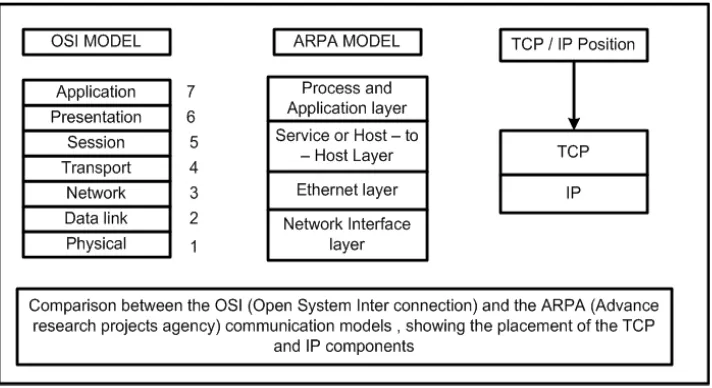
The standard that has created an enormous amount of interest in the past few years is Ethernet. Other protocol, which fits onto Ethernet extremely well, is TCP/IP, and being derived from the Internet is very popular and widely used.
5.2.
Open Systems Interconnection (OSI) model
Figure 5. 1
OSI model representation: two hosts interconnected via a router
The OSI model is useful in providing a universal framework for all communication systems. However, it does not define the actual protocol to be used at each layer. It is anticipated that groups of manufacturers in different areas of industry will collaborate to define software and hardware standards appropriate to their particular industry. Those seeking an overall framework for their specific communications’ requirements have enthusiastically embraced this OSI model and used it as a basis for their industry specific standards.
5.2.1. Protocols
As previously mentioned, the OSI model provides a framework within which a specific protocol may be defined. A protocol, in turn, defines a frame format that might be made up of various fields as follows.
Figure5. 2
Basic structure of an information frame
5.3. RS-232
interface
standard
The RS-232 interface standard (officially called TIA-232) defines the electrical and mechanical details of the interface between Data Terminal Equipment (DTE) and Data Communications Equipment (DCE), which employ serial binary data interchange. The current version of the standard refers to DCE as Data Circuit-terminating Equipment.
Figure5. 3
A typical serial data communications link
The RS-232 standard consists of three major parts, which define:
• Electrical signal characteristics
• Mechanical characteristics of the interface
• Functional description of the interchange circuits
5.3.1. Half-duplex operation of RS-232
The following description of one particular mode of operation of the RS-232 interface is based on half-duplex data interchange. The description encompasses the more generally used full-duplex operation.
Figure 5. 4
Figure 5. 4 shows the operation with the initiating user terminal, DTE, and its associated modem, DCE, on the left of the diagram and the remote computer and its modem on the right.
Full-duplex operation requires that transmission and reception must be able to occur simultaneously. In this case, there is no RTS/CTS interaction at either end. The RTS and CTS lines are left ON with a carrier to the remote computer.
5.4. Fiber
Optics
Fiber optic communication uses light signals guided through a fiber core. Fiber optic cables act as waveguides for light, with all the energy guided through the central core of the cable. The light is guided due to the presence of a lower refractive index cladding around the central core. Little of the energy in the signal is able to escape into the cladding and no energy can enter the core from any external sources. Therefore the transmissions are not subject to any electromagnetic interference.
The core and the cladding will trap the light ray in the core, provided the light ray enters the core at an angle greater than the ‘critical angle’. The light ray will then travel through the core of the fiber, with minimal loss in power, by a series of total internal reflections. Figure 5. 5 illustrates this process.
Figure 5. 5
Light ray traveling through an optical fiber
5.4.1. Applications for fiber optic cables
Fiber optic cables offer the following advantages over other types of transmission media:
• Light signals are impervious to interference from EMI or electrical
crosstalk
• Light signals do not interfere with other signals
• Optical fibers have a much wider, flatter bandwidth than coaxial
cables and equalization of the signals is not required
• The fiber has a much lower attenuation, so signals can be transmitted
much further than with coaxial or twisted pair cable before amplification is necessary
• Optical fiber cables do not conduct electricity and so eliminate
problems of ground loops, lightning damage and electrical shock
• Fiber optic cables are generally much thinner and lighter than copper
cables
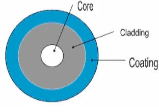
5.4.2. Fiber optic cable components
The major components of a fiber optic cable are the core, cladding, coating (buffer), as shown in Figure 5. 6. Some types of fiber optic cable even include a conductive copper wire that can be used to provide power to a repeater.
Figure 5. 6
Fiber optic cable components
The fiber components include:
• Fiber core
• Cladding
• Coating (buffer)
• Strength members
• Cable sheath
There are four broad application areas into which fiber optic cables can be classified: aerial cable, underground cable, sub-aqueous cable and indoor cable.
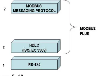
5.5. Modbus
Modbus Messaging protocol is an Application layer (OSI layer 7) protocol that provides client/server communication between devices connected to different types of buses or networks. The Modbus Messaging protocol is only a protocol and does not imply any specific hardware implementation. Also note that the Modbus Messaging protocol used with Modbus Serial is the same one used with Modbus Plus and Modbus TCP.
Modbus messaging is based on a client/server model and employs the following messages:
• Modbus requests, i.e. the messages sent on the network by the clients
to initiate transactions. These serve as indications of the requested services on the server side
• Modbus responses, i.e. the response messages sent by the servers.
These serve as confirmations on the client side
Figure5. 7
Modbus transaction
The Application Data Unit (ADU) structure of the Modbus protocol is shown in the Figure 5.8.
Figure5. 8
Modbus serial ADU format
Modbus functions can be divided into four groups or ‘Conformance Classes’. The Function Codes are normally expressed in decimal; the hexadecimal equivalents are shown in brackets.
Conformance Class 0 is the minimum set of useful commands for both controllers and target devices. Note that the descriptions of certain commands have changed over the years, for this reason both the current and historical (‘classic’) descriptions are given here.
Function Code Current terminology Classic terminology
3 (0x03) Read multiple registers Read holding registers
16 (0x10) Write multiple registers Preset multiple registers
Table5. 1
Conformance Class 0 commands
Conformance Class 1 comprises an additional set of commands, commonly implemented and interoperable.
Function Code Current terminology Classic terminology
1 (0x01) Read coils Read coil status
2 (0x02) Read input discretes Read input status
4 (0x04) Read input registers Read input registers
5(0x05) Write coil Write single register
7(0x07) Read exception status
Read exception status
Table5. 2
Conformance Class 1 commands
Function Code 7 usually has a different meaning for each PLC family.
Conformance Class 2 comprises the data transfer functions needed for routine operations and supervision. These include, but are not limited to:
Function Code Current terminology Classic terminology
15 (0x0F) Force multiple coils Force multiple coils
22 (0x16) Mask write register Mask write register
23 (0x17) Read/write registers Read/write registers
Table5. 3
Conformance Class 2 commands
There are also others such as Function Code 20 (read general reference), Function Code 21 (write general reference) and Function Code 24 (read FIFO queue) but they are considered to be outside the ambit of this section.
• Machine/vendor/network specific functions are those that, although
being mentioned in the Modbus manuals, are not appropriate for interoperability because they are too machine-dependent. These include Function Codes such as 9 (program: Modicon 484), 10 (poll: Modicon 484) and 19 (reset communications link: Modicon 884/u84).
The following table summarizes the relationship of some of the more commonly used commands and the input/output addresses. The descriptions use the current rather than the classic terminology.
Data type Absolute
Discrete inputs 10001 to 19999 0 to 9998 02 Read input discretes
Input registers 30001 to 39999 0 to 9998 04 Read input registers
Holding registers 40001 to 49999 0 to 9998 03 Read multiple registers
Holding registers 40001 to 49999 0 to 9998 06 Write single register
Holding registers 40001 to 49999 0 to 9998 16 Write multiple registers
– – – 07 Read exception status
– – – 08 Loopback diagnostic
test
Table5. 4
Modicums addresses and Function Codes
5.5.1.1. Example of Function Code 2: Read input discretes
the request frame consists of the protocol address of the first discrete input followed by the number of discrete inputs to be read. The data field of the response frame consists of a count of the discrete input data bytes followed by that many bytes of discrete input data.
The discrete input data bytes are packed with one bit for the status of each consecutive discrete input. The least significant bit of the first discrete input data byte conveys the status of the first input read (i.e. the one with the lowest address). If the number of discrete inputs read is not an even multiple of eight, the last data byte will be padded with zeros on the high end. If there are more than eight bits in the response, the second byte will contain the next bits and so on. Once again this is not consistent with a big-endian approach.
In the following example, the controller requests the status of discrete inputs with protocol addresses 0x0000 and 0x0001 i.e. addresses 10001 and 10002 PLC. The target device’s response indicates that discrete input 10001 is OFF and discrete input 10002 is ON (Figure5. 9).
• ‘Reference number’ refers to the input discrete with the lowest address
• ‘Bit count’ refers to the number of input discretes (‘number of points’)
to be read and can vary between 1 and 2000
• ‘Byte count’ refers to the number of bytes required to return the
requested input discrete values and is calculated as ((bit count + 7) / 8)
‘Bit values’ refer to the actual values of the individual inputs or ‘input data’
Figure5. 9
Example: FC02-reading input discretes
5.5.2. Modbus Plus