Model Checking Markov Reward Models
with Impulse Rewards
Maneesh Khattri Mhd. Reza M. I. Pulungan
A thesis submitted to the department of Computer Science of the University of Twente for the partial fulfillment
of the requirements of the degree of Master of Science in Telematics
Graduation Committee:
Dr. ir. Joost-Pieter Katoen (mtd.) Dipl. Inform. Lucia Cloth
Abstract
A Markov Reward Model (MRM) is a Stochastic Process satisfying the Markov property. MRMs have been used for the simultaneous analysis of performance and dependability issues of computer systems, sometimes referred to as performability. Previous work for Model Checking MRMs [Bai00, Bai02, Hav02] is restricted to state-based reward rates only. However, greater insight into the operation of systems can be obtained when impulse rewards are incorporated in these models which express the instantaneous cost imposed with the change of state of systems. The main aim of this thesis is to enable Model Checking of MRMs with impulse rewards. In this thesis methods for Model Checking MRMs have been extended for the incorporation of impulse rewards. To that end, the syntax and semantics of the temporal logic CSRL (Continuous Stochastic Reward Logic) have been adapted and algorithms have been developed and implemented that allow for the automated verification of properties expressed in that logic.
Acknowledgements
We thank our supervisors Dr. ir. Joost-Pieter Katoen and Dipl. Inform. Lucia Cloth for their support and guidance during the course of this project work. We especially extend our gratitude to Dr. ir. Joost-Pieter Katoen for directing us towards a project, for patiently reading versions of this report and helping us in improving it.
We also thank Dr. ir. Henk Alblas, Drs. Jan Schut and Ms. Belinda Jaarsma Knol for helping us on many occasions during our stay in the Netherlands. We’re indebted to family members and friends for their encouragement and help.
Contents
Abstract iii
List of Tables ix
List of Figures xi
1 Introduction 1
1.1 Markov Reward Model . . . 1
1.2 Model Checking . . . 2
1.3 Motivation . . . 3
1.4 Objective . . . 3
1.5 Structure . . . 4
2 Markov Processes 5 2.1 Stochastic Processes . . . 5
2.2 Markov Processes . . . 6
2.3 Discrete-Time Markov Chains . . . 7
2.3.1 Transient Analysis . . . 8
2.3.2 Steady-State Analysis . . . 9
2.4 Continuous-Time Markov Chains . . . 9
2.4.1 Transient Analysis . . . 10
2.4.2 Steady-State Analysis . . . 11
2.5 Labeled Continuous-Time Markov Chain . . . 11
2.5.1 Atomic Propositions . . . 12
2.5.2 Interpretation Function: Labeling (Label) . . . 12
3 Markov Reward Model (MRM) 15 3.1 Markov Reward Model . . . 15
3.2 Paths in MRM . . . 17
3.3 Probability of Paths . . . 19
3.4 Transient and Steady-State Probability . . . 19
3.5 MRM and Performability . . . 20
3.6 A Logic for MRMs (CSRL) . . . 20
3.6.1 Syntax of CSRL . . . 21
3.6.2 Semantics of CSRL . . . 23
3.7 Steady-State Measures . . . 24
3.8 Transient Measures . . . 26
3.8.1 NeXt Formula . . . 26
3.8.2 Until Formula . . . 27
4 Model Checking MRMs 29 4.1 The Model Checking Procedure . . . 29
4.2 Model Checking Steady-State Operator . . . 30
4.3 Model Checking Transient Measures . . . 32
4.3.1 Next Formulas . . . 32
4.3.2 Until Formulas . . . 33
4.4 Numerical Methods . . . 37
4.4.1 Discretization . . . 37
4.4.2 Uniformization for MRMs . . . 38
4.5 Discretization Applied to Until Formulas . . . 42
4.5.1 Computational Requirements . . . 43
4.6 Uniformization Applied to Until Formulas . . . 43
4.6.1 Error Bounds . . . 44
4.6.2 Generation of Paths and Path Probabilities . . . 44
4.6.3 Computation of Conditional Probability . . . 46
4.6.4 Computational Requirements . . . 50
5 Experimental Results 51 5.1 Implementation . . . 51
5.2 Results without Impulse Rewards . . . 52
5.3 Results with Impulse Rewards . . . 53
5.3.1 Experimental Setup . . . 53
5.3.2 Results by Uniformization . . . 54
5.3.3 Results by Discretization . . . 57
6 Conclusions 59
Bibliography 61
List of Tables
5.1 Result without Impulse Rewards . . . 52
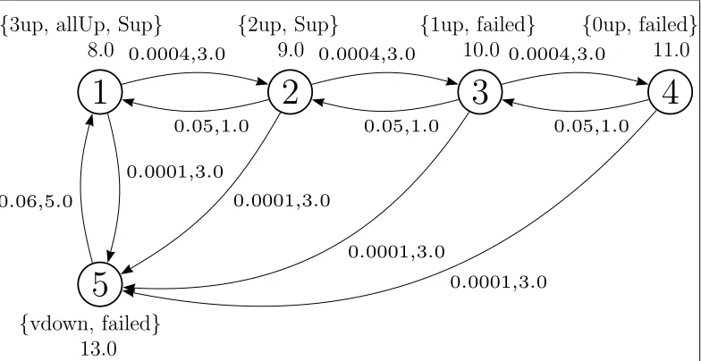
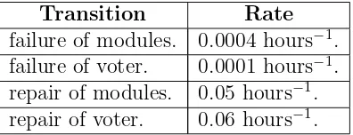
5.2 Rates of the TMR Model . . . 54
5.3 Maintaining Constant Value for Truncation Probability . . . 54
5.4 Maintaining Error Bound . . . 55
5.5 Reaching the Fully Operational State with Constant Failure Rates 56 5.6 Variable Rates . . . 57
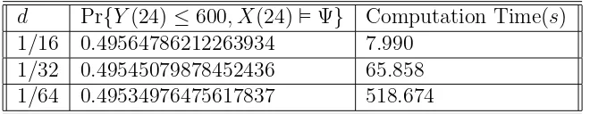
5.7 Reaching the Fully Operational State with Variable Failure Rates 58 5.8 Results by Discretization . . . 58
List of Figures
2.1 A DTMC Represented in Labeled Directed Graph . . . 7
2.2 WaveLAN Modem Modeled as a Labeled CTMC . . . 13
3.1 WaveLAN Modem Modeled as an MRM . . . 16
3.2 BSCCs in Steady-State Analysis . . . 25
4.1 WaveLAN Modem Model wherebusy-states are made absorbing . 35 4.2 WaveLAN Modem Model after Uniformization . . . 39
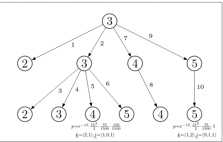
4.3 Depth First Path Generation . . . 45
5.1 Model Checker for MRMs . . . 52
5.2 Triple-Modular Redundant System . . . 53
5.3 T vs. t and E vs. t for constantw= 10−11 . . . . 55
5.4 P and T vs. Number of working modules with constant failure rates 57 5.5 P and T vs. Number of working modules with variable failure rates 58
Chapter 1
Introduction
This chapter presents the motivation, objective and structure of this thesis. A brief introduction to Markov Reward Models is presented in section 1.1. Section
1.2 gives a short overview of Model Checking. The motivation behind this thesis is presented in section 1.3. In section 1.4, the objective of this project is stated and section 1.5 describes the structure of this thesis.
1.1
Markov Reward Model
Many events occur in a disorderly or random fashion. For instance the arrival of a customer to an airline counter or the time it will take to serve the customer. In mathematics such events are described by random functions for which if the value of the function is given at a certain point of time, its future value can only be determined with a certain probability and not precisely. Such functions to represent random events are referred to as Stochastic Processes [How71, Hav98]. One special class of Stochastic Processes is referred to as theMarkov Process. A Markov Process is essentially a Stochastic Process which satisfies the Markov Property. The Markov Property states that “given the present state, the knowl-edge of the past states does not influence the future state.” This is sometimes referred to as the memoryless property. A Markov Chain is a Markov Process whose state space is finite or countably infinite.
A Markov Reward Model (MRM) is such a Markov Chain. It is augmented with a reward assignment function. The reward assignment function assigns a
state-based reward rateto each state such that the residence time in a state entails the accumulation of overall reward gained based on the state-based reward rate. The reward assignment function also assigns animpulse reward to each transition such that the occurrence of the transition results in a gain in the overall reward governed by the impulse reward assigned to the transition.
The application of Markov Reward Models to computer systems can be traced back to the work of Professor John F. Meyer of the University of Michigan, Ann Arbor [Mey80] which concerns the simultaneous analysis ofperformance and
dependability of computer systems. Whilst performance in computer systems is
the efficacy by which the system delivers services under the assumption that the services delivered conform to the specification, dependability is the ability of the system to deliver services that conform to the specification. Although these two issues may be analyzed independently, simultaneous analysis becomes imperative when the performance of the systemdegrades under the presence of behavior that does not conform to the specification. This analysis is sometimes referred to as
performability [Mey95].
The definition of theperformability measure is based on aperformability vari-able (Y). The performability variable is realized over abase stochastic model and incorporates an utilization interval and an accomplishment set in which the per-formability variable takes its values. An example of such an accomplishment set is the set of all non-negative real numbersR≥0. The performability measure for a
subset of the accomplishment set is then the probability that the performability variable interpreted over the stochastic process takes values in the subset. For instance, a subset of the accomplishment set R≥0 is [0, y],y∈R≥0.
The accumulated reward over an MRM in a finite interval can be considered to be a performability variable. Then performability over an MRM for a finite interval [0, t] and for a set [0, y], y ∈ R≥0 is defined as the probability that the
accumulated reward is in [0, y] over a utilization interval [0, t].
1.2
Model Checking
Model Checking [Cla99, Kat02] is aformal verification strategy. The verification of systems requires first a precisespecification of the system. A model of the system is then constructed whose behavior should correspond to the specification. Once such a model is available, statements about functional correctness of the system can be made. The specification of these statements is made in mathematical logic such as temporal logic interpreted over the model. Subsequently, a set of statements about the functional correctness of the system are made.
1.3. MOTIVATION 3
1.3
Motivation
In recent times as performability requirements on computer systems become more acute, models based on MRM are gaining more importance and so do verification techniques for these models. This is the inspiration to investigate model checking applied to the field of performability. Many qualitative and quantitative state-ments can be made about systems modeled in terms of such MRM by means of Model Checking. Previous work for Model Checking MRMs [Bai00, Bai02, Hav02] is restricted to state-based reward rates only. However, greater insight into the operation of systems can be obtained when impulse rewards are incorporated in these models which express the instantaneous cost imposed with the change of state of systems.
The occurrence of this instantaneous cost in terms of energy consumption can be observed in modern-day cellular phones. The phone periodically moves to an idle state. It then stays in such a state continuously unless a call is initiated or received or if a location hand-over becomes necessary. If a call is received then the phone has to transition to a state where it can handle the call. During this transition instantaneous costs related to tasks such as preparing to ring the ringer are endured. This behavior of accumulating instantaneous costs can be modeled by impulse reward functions.
This ability to model instantaneous costs is the motivation to extend Model Checking procedures defined for MRMs with only state-based reward rates to
include impulse reward functions. A further motivation is to develop efficient and numerically stable algorithms for model checking MRMs.
1.4
Objective
To develop modeling formalisms and practical algorithms for model checking Markov Reward Models with state-based reward rate and impulse rewards. To fulfill this objective the following tasks are distinguished:
1. Background study of Markov Processes, Markov Reward Models and Per-formability measures.
2. Extension of definitions, model and logic to incorporate impulse rewards. 3. Survey of numerical methods to compute measures defined over MRMs. 4. Development and implementation of algorithms for Model Checking MRMs. 5. Development of an example application which is modeled as an MRM and
performing experiments with the example.
1.5
Structure
This thesis is organized as follows:
Chapter 2: Markov Processes describes background theory of Markov Pro-cesses. It presents a brief introduction to Stochastic Processes, Markov Processes and Discrete & Continuous-Time Markov Chains.
Chapter 3: Markov Reward Model (MRM) describes Markov Reward Mod-els. It presents the formal definition of MRMs and measures interpreted over these MRMs. Subsequently a logic (CSRL) to specify properties over MRMs is presented.
Chapter 4: Model Checking MRMs describes the model checking procedure to check the validity of properties specified in CSRL interpreted over MRMs. Numerical methods which have been developed to check the validity of CSRL properties are presented. This constitutes the main part of this thesis.
Chapter 5: Experimental Results describes the implementation of model checking procedures and several experiments using this implementation. It also presents a comparison of the performance of the numerical methods with existing methods for models with only state-based reward rates.
Chapter 2
Markov Processes
This chapter presents background theory of Markov Processes. A brief introduc-tion to Stochastic Processes is presented in section 2.1. Section 2.2 gives an overview of Markov Processes. Discussion about Discrete and Continuous-Time Markov Chains is presented in section 2.3 and in section 2.4 respectively. Sec-tion 2.5 discusses Continuous-Time Markov Chains augmented with a labeling function.
2.1
Stochastic Processes
A Stochastic Process is a collection of random variables{X(t)|t∈ T }indexed by a parameter t which can take values in a set T which is the time domain. The values that X(t) assumes are called states and the set of all possible states is called the state space I. Both set I and T can be discrete or continuous, leading to the following classification:
1. Discrete-state discrete-time stochastic processes can be used for instance to model the number of patients that visit a physician where the number of patients represents states and time is measured in days.
2. Discrete-state continuous-time stochastic processes can be used for instance to model the number of people queueing in an airplane ticketing counter where the number of people in the queue represents states.
3. Continuous-state discrete-time stochastic processes can be used for instance to model the volume of water entering a dam where the volume of water entering the dam represents states and time is measured in days.
4. Continuous-state continuous-time stochastic processes can be used for in-stance to model the temperature of a boiler where the temperature of the boiler represents states.
At a particular time t′ ∈ T, the random variable X(t′) may take different
values. The distribution function of the random variable X(t′) for a particular
t′ ∈ T is defined as:
F(x′, t′) = Pr{X(t′)≤x′},
which is also called the cumulative density function of the random variable or the first-order distribution of the stochastic process {X(t)|t∈ T }. This function can be extended to the n-th joint distribution of the stochastic process as follows:
F(x′, t′) = Pr{X(t′1)≤x′1, . . . , X(t′n)≤x′n},
where x′ and t′ are vectors of size n, x′
i ∈ I and t′i ∈ T for all 1≤i≤n.
Anindependent process is a stochastic process where the state being occupied at a certain time does not depend on the state(s) being occupied in any other time-instant. Mathematically, an independent process is a stochastic process whose n-th order joint distribution satisfies:
F(x′, t′) = n
Y
i=1
F(x′i, t′i) = n
Y
i=1
Pr{X(t′i)≤x′i}.
A stochastic process can also be a dependent process in which case some form of dependence exists among successive states.
2.2
Markov Processes
One form of a dependent process in which there is a dependence only between two successive states is called a Markov process. Such dependence is called Markov dependence or first-order dependence. A stochastic process {X(t)|t ∈ T } is a Markov process if for any t0 < t1 <· · ·< tn< tn+1, the distribution of X(tn+1),
given X(t0),· · · , X(tn), only depends on X(tn), or mathematically:
Pr{X(tn+1)≤xn+1|X(t0) = x0, . . . , X(tn) =xn}= Pr{X(tn+1)≤xn+1|X(tn) =xn},
which is referred to as the Markov property. This is to say that the immedi-ate future stimmedi-ate in a Markov process depends only on the stimmedi-ate being occupied currently.
A Markov process is called time-homogeneous if it is invariant to time shifts which means that the behavior of the process is independent of the time of ob-servation. For any t1 < t2, x1 and x2:
Pr{X(t2)≤x2|X(t1) =x1}= Pr{X(t2−t1)≤x2|X(0) =x1}.
2.3. DISCRETE-TIME MARKOV CHAINS 7
2.3
Discrete-Time Markov Chains
A Discrete-Time Markov Chain (DTMC) is a stochastic process such that the state spaceI and the setT are both discrete, and the stochastic process satisfies the Markov property, which in the discrete-state and discrete-time case is defined as:
Pr{Xn+1) =in+1|X0 =i0,· · · , Xn =in}= Pr{Xn+1 =in+1|Xn =in},
whereT ={0,1,2, . . .} and i0, . . . in+1 ∈ I.
Let pi(n) denote the probability of being in state i at time n, and the con-ditional probability pj,k(m, n) = Pr{Xn = k|Xm = j} denote the probability of being in state k at time n, given that at time m the DTMC is in state j. Since in time-homogeneous Markov chains, the transition probabilities only depend on the time difference, this conditional probability can be written as pj,k(l) = Pr{Xm+l =k|Xm =j}, which is called thel-step transition probability. Hence, thel-step transition probabilitypj,k(l) denotes the probability of being in statek afterl steps given that the current state isj. The 1-step probabilities are pj,k(1) or simply pj,k and the 0-step probabilities are the initial distribution of the DTMC. A DTMC is described by the initial probabilitiesp(0) and the 1-step probabilities, which is represented by the state-transition probability matrix P.
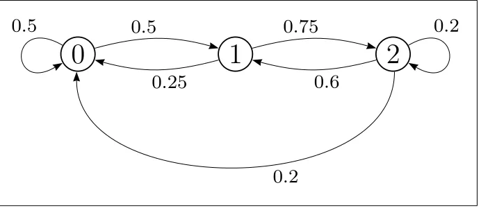
Example 2.1 A DTMC can be conveniently represented graphically as a labeled directed graph. The vertices in the graph represent states in the DTMC and the name of the state is in the vertex that represents the state. A transition is represented by an edge in the graph. The probability of a transition is placed near the edge representing the transition in question. Figure 2.1 is an example of such a graph.
0
1
2
0
.
5
0
.
5
0
.
25
0
.
75
0
.
6
0
.
2
0
.
2
Figure 2.1: A DTMC Represented in Labeled Directed Graph
probability, for instance, transition from state 0 to state 1 occurs with probability
0.5. From the figure the 1-step probabilities are given by:
P =
0.5 0.5 0 0.25 0 0.75
0.2 0.6 0.2
.
The Markov property can only be satisfied if the state residence time in the DTMC has a memoryless discrete distribution. Since the geometric distribution is the only memoryless discrete distribution, it follows that the state residence time in a DTMC is geometrically distributed. Hence, for every state i∈ I in the DTMC a non-negative real valuePi,i = 1−Pi6=jPi,j, is associated such that the residence time distribution in state i (the probability to reside in state i for n steps) is:
Fi(n) = (1−Pi,i)·Pni,i−1, n≥0.
2.3.1
Transient Analysis
Transient analysis aims at determining the probability with which the DTMC occupies a state after a given number of observation steps have occurred. This probability is referred to as the state occupation probability. These state occupa-tion probabilities are given by:
p(n) = p(0)·Pn,
where p(0) is the initial distribution of the DTMC and P is the state-transition probability matrix. The state occupation probabilities, which is contained inp(n) express the transient behavior of the DTMC.
Example 2.2 Using the DTMC presented in figure 2.1,and p0(0) = 1; pi(0) = 0
for i= 1,2; the state occupation probabilities after 3 steps are as follows:
p(3) =p(0)·P3 =h1 0 0i·
0.5 0.5 0 0.25 0 0.75
0.2 0.6 0.2
3
=h0.325 0.412 5 0.262 5i.
These state occupation probabilities describe the probabilities of ending in states after 3 steps starting from state 0. For instance, after 3 steps, starting from state 0, the DTMC will be in state 2 with probability 0.2625. State occupa-tion probabilities after more number of steps have elapsed can also be obtained. For instance the state occupation probabilities after15and25steps are as follows:
2.4. CONTINUOUS-TIME MARKOV CHAINS 9
In the previous example it can be observed that after a certain number of steps, the state occupation probabilities converge. It would be interesting to know if the converged probabilities can be determined directly since for some measures these converged probabilities will suffice to describe the behavior of the DTMC. However, such converged probabilities do not exist for all DTMC. The conditions under which these converged probabilities exist are presented in [Hav98].
2.3.2
Steady-State Analysis
The steady-state analysis aims at determining the state occupation probabil-ities after an unbounded number of steps have occurred in a DTMC: vi = limn→∞pi(n), which are called the steady-state probabilities. If this limit exists,
these steady-state probabilities are described by a system of linear equations: v =v·P,Xivi = 1,0≤vi ≤1.
Vector v is referred to as the steady-state probability vector of the DTMC, which describes the steady-state distribution of the DTMC.
Example 2.3 Using the DTMC presented in figure 2.1, in a long run, after infinite steps occur in the DTMC, the state occupation probabilities are given by the steady-state probabilities. For the DTMC, the steady-state probabilities are:
v =v·
0.5 0.5 0 0.25 0 0.75
0.2 0.6 0.2
,
X
ivi = 1,0≤vi ≤1⇒v =
h
14 45
16 45
1 3
i
.
These steady-state probabilities can be interpreted as the probabilities of dis-covering that the DTMC is in some state after it has been running for a long time. They can also be interpreted as the fraction of time the DTMC stays in some state in the long run. Thus for the example, it can be said that after a long running time the DTMC will be in state 2 with probability 1
3 or the fraction of
running time that the DTMC spends in state 2 is 13.
2.4
Continuous-Time Markov Chains
A Continuous-Time Markov Chain (CTMC) is a stochastic process such that the state space I is discrete, the set T is continuous, and the stochastic process satisfies the Markov property namely:
Pr{X(tn+1) =xn+1|X(t0) =x0,· · · , X(tn) =xn}= Pr{X(tn+1) =xn+1|X(tn) =xn}.
every statei∈ I in the CTMC a random variable with parameter a non-negative real value µi, referred to as the rate, is associated such that the residence time distribution in state i is:
Fi(t) = 1−e−µi·t, t ≥0.
Beside the state residence time distribution with rate µi, several delays de-pending on the number of transitions are associated with every state with rate
Ri,j. The total rate of taking an outgoing transition from stateiisE(i) = PjRi,j. Note that the rate of residence in statei is nowµi =E(i). These delays can con-veniently be represented in a rate matrix R.
The operation of CTMCs can be imagined as follows, at any given instant the CTMC is said to be in one of the states. Let the CTMC enter state i at some observation instant. Subsequently, it will make a transition to one of the states j after residing in statei for a negative exponentially distributed interval of time given by the following distribution:
Fi,j(t) = 1−e− i,j·t.
Since the delays assigned to various transitions from state i can be different, the transition corresponding to the fastest rate will take the shortest time to take place. Hence at the observation instant all transitions from statei are said to be in arace condition. Due to this property the probability that a certain transition i→j is successful in relation to other transitions from state i is:
P(i, j) = PRi,j
kRi,k .
Consequently, the probability of moving from state i to a statej within time t is given by P(i, j)·(1−e−E(i)·t). For most measures defined over CTMCs the specification of a CTMC involves the specification of the initial probability vector p(0) and the rate matrixR only.
2.4.1
Transient Analysis
For many measures that are defined over CTMCs it is interesting to know the probability with which the CTMC occupies a state after a given observation inter-val has elapsed. This probability is referred to as thestate occupation probability. The analysis used to determine the state occupation probabilities in this manner is called transient analysis of CTMCs. These state occupation probabilities are described by a linear system of differential equations:
p′(t) =p(t)·Q, (2.1)
where
2.5. LABELED CONTINUOUS-TIME MARKOV CHAIN 11
is the infinitesimal generator matrix.
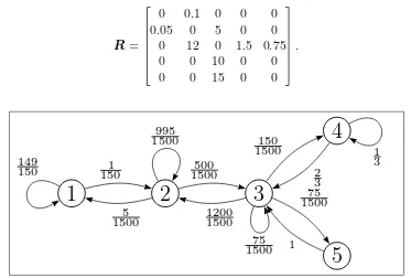
In many practical situations, uniformization is used to perform transient analysis of CTMC by analyzing the uniformized Discrete Time Markov Chain (DTMC). To generate the uniformized process of the CTMC, specified by ini-tial probability distribution p(0) and rate matrix R, first obtain the infinitesimal generator matrix Q:
Q=
Q1,1 Q1,2 · · · Q1,n Q2,1 Q2,2 · · · Q2,n
· · · ·
Qn,1 Qn,2 · · · Qn,n
where
Qi,i =−
n
X
j=1
Qi,j,
a rate of residence Λ is assigned to each state where Λ≥maxi(−Qi,i). The 1-step probability matrix for the uniformized process is found in the following fashion:
P =I+Q
Λ whereI is an Identity matrix of cardinality (n×n).
Once such a uniformized process is available, let {Nt : t ≥ 0} be a Poisson process with rate Λ,p(t), the distribution of state occupation probability at time t, is:
p(t) =
∞
X
i=0
e−Λt(Λt)i
i! ·p(0)·P i
. (2.2)
2.4.2
Steady-State Analysis
Consider a CTMC specified by an initial probability distribution p(0) and a rate matrix R. For many measures defined over such a CTMC it suffices to consider the steady-state distribution. The steady-state analysis aims at determining the state occupation probabilities after an unbounded observation interval is allowed to elapse: pi = limt→∞pi(t). For finite CTMC this limit always exists; hence
from equation (2.1) p′(t) = 0. Consequently, these steady-state probabilities are
described by a system of linear equations: p·Q= 0,X
i∈I
pi = 1. (2.3)
When the steady-state distribution depends on the initial-probability distri-bution then a graph analysis to determine the bottom-strongly connected com-ponents can be performed. This is elaborated upon in chapter 3.
2.5
Labeled Continuous-Time Markov Chain
2.5.1
Atomic Propositions
Atomic propositions are the most elementary statements that can be made, can-not be further decomposed and can be justified to betrueorfalse. For instance, “It is Sunday” is an atomic proposition. The finite set of all atomic propositions is referred to as AP. The selection of such a set AP determines the qualitative aspects that can be expressed about a system.
2.5.2
Interpretation Function: Labeling (Label)
Label : S −→ 2AP: A labeling function Label assigns to each state s a set of atomic propositionsLabel(s)∈AP that are valid (true) in states. The function Label indicates which atomic propositions are valid in which states. A statesfor which the atomic propositionp∈AP is valid i.e. p∈Label(s) is called ap-state.
Definition 2.1 A Continuous-Time Markov Chain (CTMC) C is a three-tuple
(S,R, Label) where S is a finite set of states, R: S×S −→R≥0 is a function.
R is called the rate matrix of the CTMC, where Rs,s′ is the rate of moving from
state s to s′. It is said that there is a transition from state s to state s′ if and only if Rs,s′ >0. Label:S −→2AP is a labeling function.
The total rate of taking an outgoing transition from state s ∈ S is given by E(s) = Ps′∈SRs,s′. The probability of moving from state s to any state within time t is (1−e−E(s)t). The probability of moving from state s to a state s′ is:
P(s, s′) = Rs,s′ E(s).
The probability of making a transition from state s to s′ within time t is
Rs,s′
E(s) ·(1−e
−E(s)·t). Note that this definition of a CTMC is different from the original definition of a CTMC in the sense that self-transitions are allowed to occur. This implies that after a negative exponentially distributed residence time in a state has elapsed the CTMC may transition to the same state.
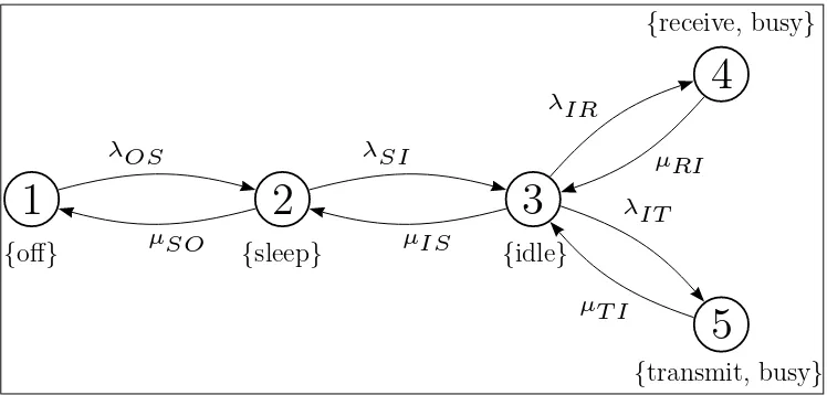
Example 2.4 Consider a WaveLAN modem which is designed to be energy- effi-cient. Typical operating modes in such an interface are off, sleep,idle, receiveand
2.5. LABELED CONTINUOUS-TIME MARKOV CHAIN 13
1
{off}
2
{sleep}
3
{idle}
4
{receive, busy}
5
{transmit, busy}
λOS µSO λSI µIS λIR µRI λIT µT I
Figure 2.2: WaveLAN Modem Modeled as a Labeled CTMC
This CTMC can be specified as C = (S,R, Label) where S ={1,2,3,4,5},
R=
0 λOS 0 0 0
µSO 0 λSI 0 0
0 µIS 0 λIR λIT
0 0 µRI 0 0
0 0 µT I 0 0
; and
Label(1) = {off},
Label(2) = {sleep},
Label(3) = {idle},
Label(4) = {receive,busy},
Label(5) = {transmit,busy}. From the rate matrix, the total rate of taking an outgoing transition for each state s∈S (E(s)) can be calculated:
E(1) =λOS,
E(2) =λSI +µSO,
E(3) =λIR+λIT +µIS,
E(4) =µRI,
E(5) =µT I.
Chapter 3
Markov Reward Model (MRM)
This chapter presents the definition of Markov Reward Model and a logic for the specification of properties over such MRM. The definition of MRM is presented in section3.1. Section 3.2 describes paths in an MRM. In section 3.3, the proba-bility measure defined over paths in MRM is described. Section3.4presents state occupation probabilities. In Section 3.5, the definition of performability and its interpretation over MRMs is presented. A logic for the specification of properties over such MRM is presented in section 3.6. Characterization of steady-state and of transient measures is described in section 3.7 and in section 3.8 respectively.
3.1
Markov Reward Model
A Markov Reward Model is formally defined as:
Definition 3.1 (Markov Reward Model (MRM)) A Markov Reward Model (MRM) M is a three-tuple ((S,R, Label), ρ, ι) where (S,R, Label) is the un-derlying labeled CTMC C, ρ : S −→ R≥0 is the state reward structure, and
ι : S ×S −→ R≥0 is the impulse reward structure such that if Rs,s > 0 then
ι(s, s) = 0.
An MRM is a labeled CTMC augmented with state reward and impulse reward structures. The state reward structure is a function ρ that assigns to each state s ∈ S a reward ρ(s) such that if t time-units are spent in state s, a reward of ρ(s)·t is acquired. The rewards that are defined in the state reward structure can be interpreted in various ways. They can be regarded as the gain or benefit acquired by staying in some state and they can also be regarded as the cost spent by staying in some state.
The impulse reward structure, on the other hand, is a function ι that assigns to each transition fromstos′, wheres, s′ ∈S andR
s,s′ >0, a rewardι(s, s′) such that if the transition from s tos′ occurs, a reward of ι(s, s′) is acquired. Similar
to the state reward structure, the impulse reward structure can be interpreted in various ways. An impulse reward can be considered as the cost of taking a transition or the gain that is acquired by taking the transition.
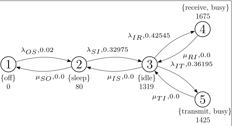
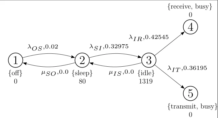
Example 3.1 Back to the WaveLAN modem example in the previous chapter, the given labeled CTMC can be extended to an MRM by augmenting it by state reward and impulse reward structures.
1
{off}
0
2
{sleep}
80
3
{idle}
1319
4
{receive, busy}
1675
5
{transmit, busy}
1425
λOS ,0.02
µSO,0.0
λSI ,0.32975
µIS ,0.0
λIR,0.42545
µRI ,0.0
λIT ,0.36195
µT I ,0.0
Figure 3.1: WaveLAN Modem Modeled as an MRM
The state reward and impulse reward structures in this example are interpreted as cost in terms of energy consumption. A WaveLAN modem, as described in [Pau01], typically consumes 1675 mW while transmitting,1425 mW while receiv-ing,1319 mW while being idle and 80mW while in sleep mode. This information is used to develop the state reward structure as follows:
ρ(1) = 0 mW, ρ(2) = 80 mW,
ρ(3) = 1319 mW, ρ(4) = 1675 mW,
ρ(5) = 1425 mW.
It is also described that transitions from sleep to idle take 250 µs with the power consumption of the idle state. It is also noted that 254 µs is required before the payload is transmitted. It is further assumed that the same duration of time is required before a payload can be received. Similarly the transition from off to sleep is assumed to take 250 µs with the power consumption of the sleep state. These observations are interpreted as impulse rewards, thus for defining the impulse rewards the transitions are assumed to be instantaneous. Hence the impulse reward structure is as follows:
ι(1,2) = 80·250·10−6 = 0.02 mJ, ι(3,4) = 1675·254·10−6 = 0.425 45 mJ,
ι(2,1) = 0 mJ, ι(4,3) = 0 mJ,
ι(2,3) = 1319·250·10−6 = 0.32975 mJ, ι(3,5) = 1425·254·10−6 = 0.361 95 mJ,
3.2. PATHS IN MRM 17
Figure 3.1 presents the labeled directed graph of the MRM described in the above example. In addition to the states and transitions that are represented by vertices and edges respectively, the labeled directed graph of an MRM also contains representations of label sets, state rewards and impulse rewards. The label set and state reward of a state are placed, in that order, near the vertex representing the state. The impulse reward of a transition is placed near the edge representing the transition after the rate of the transition.
Definition 3.2 (Absorbing State in an MRM) A state s ∈ S in an MRM M= ((S,R, Label), ρ, ι) is absorbing if and only if Rs,s′ = 0 for all s′ ∈ S.
3.2
Paths in MRM
During its running time, an MRM makes transitions from states to states. Infor-mally, the sequence of the states that the MRM resides is called a path. In this section the concept of a path in MRMs is formalized. This concept provides a tool to compute several measures in an MRM.
Definition 3.3 (Path in MRMs) An infinitepathσin MRMM= ((S,R, Label), ρ, ι)
is a sequence s0
t0
−→s1
t1
−→ · · ·, with si ∈S and ti ∈R>0 is the amount of time
spent in state si where i ∈ N and Rs
i,si+1 > 0 for all i. A finite path σ in M
is a sequence s0
t0
−→ s1
t1
−→ · · · tn−1
−→ sn, such that sn is an absorbing state and
Rsi,si+1 > 0 for all i < n. For finite paths that end in sn, tn =∞. For infinite
path σ, let σ[i] =si, i∈N. For finite path σ that ends in sn, σ[i] =si is only
de-fined fori≤n. The last state in the finite path σ (the (n+1)-st state) is referred to as last(σ). Two additional functions are defined over paths in MRMs:
The state being occupied at time t on path σ is defined as:
σ@t =σ[i]⇔
i−1
X
j=0
tj < t ∧
i
X
j=0
tj ≥t.
Rewards accumulated at time t in a path σ is a function yσ : R≥0 −→ R≥0
such that:
yσ(t) =ρ(σ[i])·
t−
i−1
X
j=0
tj
+
i−1
X
j=0
ρ(σ[j])·tj+ i−1
X
j=0
ι(σ[j], σ[j+1]) where σ@t=σ[i].
Thus, there are two types of paths: infinite and finite paths. An infinite path contains infinitely many transitions. In finite paths, there are a finite number of transitions, but the last state in the path is absorbing and an infinite amount of time is spent in this state. P athsM is the set of finite and infinite paths in the
MRM,P athsM(s) is the set of finite and infinite paths in the MRM that start in
For instance, path:
σ=s1 0
.5
−→s3 −→100 s2 −→2 s1 −→17 s4,
is a finite path. Hence, the last state in the path, s4, is absorbing and an infinite
amount of time is spent in this state. In this path σ[2] is the (2+1)-st state in the path, namely s2. Similarlyσ[0] = s1, σ[1] =s3, σ[3] = s1 and σ[4] = s4. σ[i]
is only defined for i≤4. last(σ) =s4, since s4 is the last state in the path.
A certain state can be identified to be occupied at a given time t on path σ assuming that time started from the initial state on the path. Then the i-th state on path σ is occupied at timet if the sum of the residence time of all states before the i-th state is less than t and the sum of the residence time of all states including the i-th state is greater than t.
In a similar fashion, rewards accumulated at time t in a path σ, yσ(t), can be obtained from the definition of path in MRMs, given that the state being occupied at time t is σ@t = σ[i]. The first addendum indicates the amount of reward accumulated due to residence in the i-th state until time t. The second addendum indicates the sum of rate rewards accumulated due to residence in states prior to the visit to the i-th state. The third addendum indicates the impulse rewards accumulated on the pathσ.
Example 3.2 Consider an infinite path in the WaveLAN modem as an MRM example as follows:
σ= 1 −→10 2−→4 3−→2 4−→3.75 3−→1 5−→2.5 3−→ · · ·5 .
The state that is occupied at time 21.75in path σ isσ@21.75 =σ[5] = 5since:
4
X
j=0
tj = 20.75<21.75 ∧
5
X
j=0
tj = 23.25≥21.75.
Further, the rewards accumulated at that time is yσ(21.75) where:
yσ(21.75) = ρ(σ[5])·
21.75−
4
X
j=0
tj
+
4
X
j=0
ρ(σ[j])·tj +
4
X
j=0
ι(σ[j], σ[j + 1]) = ρ(5)·(21.75−20.75) +ρ(1)·10 +ρ(2)·4 +ρ(3)·2 +ρ(4)·3.75
+ρ(3)·1 +ι(1,2) +ι(2,3) +ι(3,4) +ι(4,3) +ι(3,5) = 11983.25mW ·s + 1.13715 mJ = 11984.38715 mJ.
3.3. PROBABILITY OF PATHS 19
3.3
Probability of Paths
To be able to define and evaluate measures that are defined over MRMs it is necessary to obtain a probability measure over paths in the MRM. Given an MRM M= ((S,R, Label), ρ, ι), every state s∈S and s=s0 gives a probability
measure over all paths that originate in state s0 by Borel Space construction
[Bai00]. Let s0, . . . , sk ∈ S with Rsi,si+1 > 0 for 0 ≤ i < k and I0, . . . , Ik−1
be non-empty intervals in R≥0. Then, C(s0, I0, . . . , Ik−1, sk) denotes the cylinder
set consisting of all paths σ ∈ P athsM(s) such that σ[i] = si and ti ∈ Ii for
0≤i < k. LetF(P athsM(s)) be the smallest σ-algebra defined over P athsM(s)
which contains all the sets C(s, I0, . . . , Ik−1, sk) with s0, . . . , sk ranging over all
state sequences and s = s0 where Rsi,si+1 > 0 for 0 ≤ i < k and I0, . . . , Ik−1
ranges over all non-empty intervals in R≥0. Then the probability measure over
F(P athsM(s)) is defined by induction over k as follows:
Pr{C(s0)} = 1 for k = 0,
Pr{C(s, I0, . . . , Ik−1, sk, I′, s′)} = Pr{C(s, I0, . . . , Ik−1, sk)} ·P(sk, s′)·(e−E(sk)·a−e−E(sk)·b),
where a = inf(I′) and b = sup(I′) and the probability of taking the transition
from state sk to states′ within the time-interval I′ is:
Z
I′P(sk, s
′)·E(sk)·e−E(sk)·tdt=P(sk, s′)·(e−E(sk)·a−e−E(sk)·b),
where E(sk)·e−E(sk)·t is the probability density function of the state residence time in statesk at time t.
3.4
Transient and Steady-State Probability
Given an MRM M = ((S,R, Label), ρ, ι) with the underlying CTMC C. In chapter 2 for such CTMC C two kinds of state probabilities have been defined viz. the steady-state probability and the transient probability. The transient probability is the state occupation probability after a bounded time-interval t has elapsed. Let π(s, s′, t) represent the probability of starting in state s ∈ S
and reaching state s′ ∈S within t time-units. By the definition of probability of
paths this probability is formally defined as:
πM(s, s′, t) = Pr{σ ∈P athsM(s)|σ@t=s′}.
The steady-state analysis aims at determining the state occupation probabili-ties after an unbounded observation interval has elapsed. LetπM(s, s′) represent
the steady-state probability of starting in state s∈ S and reaching state s′ ∈ S.
This measure is given by:
π(s, s′) = lim t→∞π
When the underlying CTMC is strongly-connected then this probability does not depend on the initial-probability distribution and this probability is referred to as π(s′). This measure can also be defined for a set of states S′ ⊆S:
π(s, S′) =Xs′
∈S′π(s, s
′).
3.5
MRM and Performability
The definition and evaluation based on MRMs was initiated due to the need for simultaneous analysis ofperformanceanddependability of computer systems, also referred to asperformability [Mey95]. Whilst performance in computer systems is the efficacy by which the system delivers services under the assumption that the services delivered conform to the specification, dependability is the ability of the system to deliver services that conform to the specification. Although these two issues may be analyzed independently, simultaneous analysis becomes imperative when the performance of the systemdegrades under the presence of behavior that does not conform to the specification.
The Performability Measure Y is a random variable; its specification includes autilization period T, which is an interval of the time base and anaccomplishment set A, in whichY takes its values. The performability of the systemP erf(B) rel-ative to a specified Y whereB ⊆A, is defined to beP erf(B) = Pr{Y ∈B}. An example of such an accomplishment set is the set of all non-negative real numbers
R≥0. The performability measure for a subset of the accomplishment set is then
the probability that the performability variable interpreted over the stochastic process takes values in the subset. For instance, a subset of the accomplishment set R≥0 is [0, y],y∈R≥0.
Definition 3.4 (The Performability Measure Y(I)) The performability of a system, modeled by an MRM in the utilization intervalI in the time base such that the accumulated reward (accomplishment) is in J, is P erf(J) = Pr{Y(I)∈J}.
The accumulated reward over an MRM in a finite interval can be considered to be a performability variable. Then performability over an MRM for a finite interval [0, t] and for a set [0, y],y∈R≥0 is defined as the probability that the
ac-cumulated reward is in [0, y] over a utilization interval [0, t] and the performability measure is then defined to beP erf(≤r) = Pr{Y(t)≤r}.
3.6
A Logic for MRMs (CSRL)
3.6. A LOGIC FOR MRMS (CSRL) 21
over an MRM are specified in the Continuous Stochastic Reward Logic (CSRL)
[Bai00, Hav02].
The definition of such a logic provides the means for expressing requirements of the system being modeled as an MRM. The definition encapsulates two sub-components viz. the syntax and the semantics. The syntax of the logic defines precisely what constitutes a CSRL formula. It provides the means to specify properties of the system modeled as an MRM. However, the syntax alone does not explain the interpretation of these formulas over the system. This interpretation is explained by the semantics. The syntax and semantics of CSRL over MRMs with both state and impulse reward structures are as follows:
3.6.1
Syntax of CSRL
The definition of the syntax of CSRL is concerned with the development of means by which properties of systems being modeled as MRMs can be expressed. In CSRL two kinds of formulas are distinguished viz. state formulas and path for-mulas. Formulas whose validity is investigated given a state are referred to as state formulas while formulas whose validity is investigated given a path are said to be path formulas. The first step is the definition of a set of atomic propositions, AP. The definition of such a set AP determines the set of qualitative properties of the system that can be expressed. Given a set AP the following definition presents the formulas that can be expressed in CSRL:
Definition 3.5 (Syntax of Continuous Stochastic Reward Logic (CSRL))
Let p ∈ [0,1] be a real number, E ∈ {<,≤,≥, >} a comparison operator and I
andJ intervals of non-negative real numbers. The syntax of CSRL formulas over the set of atomic propositions AP is defined as follows:
tt is a state formula,
Each a∈AP is a state formula,
If Φand Ψ are state formulas then ¬Φand Φ∨Ψ are state formulas, If Φis a state formula then S p(Φ) is a state formula,
If ϕ is a path formula then is P p(ϕ) a state formula, If Φand Ψ are state formulas then XI
JΦ and ΦUJIΨ are path formulas. Interval I is a timing constraint, while interval J is a bound for the accumu-lated reward. X is called ne(X)t operator, while U is called (U)ntil operator. These formulas can be distinguished as follows:
State Formulas
2. The measure S p(Φ) is referred to as the steady-state measure. The state formula S p(Φ) asserts that the steady-state probability for the set of Φ-states meets the bound Dp.
3. The measureP p(ϕ) is referred to as thetransient probability measure. The state formulaP p(ϕ) asserts that the probability measure of paths satisfying ϕ meets the bound Dp.
Path Formulas
1. The measure XI
JΦ asserts that a transition is made to a Φ-state at time t∈I such that the accumulated reward until time t, r∈J.
2. The measure ΦUI
JΨ asserts that Ψ-formula is satisfied at some future time t ∈ I such that the accumulated reward until time t, r ∈ J and the Φ-formula is satisfied at all instants beforet.
3. Additional formulae are defined by direct consequence of the syntax of CSRL: ♦I
JΦ = ttUJIΦ and P p(IJΦ) =¬P p(♦IJ¬Φ).
Example 3.3 Some interesting measures of the WaveLAN modem example that can be expressed in CSRL are as follows:
• The probability is more than 0.5 that the system is either transmitting or receiving after a certain duration of time has elapsed. It is assumed that the system has only 50 J of energy. Then after an observation interval of
10 minutes is allowed to elapse this property is: P>0.5(ttU[0
,600] [0,50] busy).
• Energy consumption in WaveLAN can be significantly reduced if the inter-face spends most of the time in sleep mode. One way to improve this is by imposing requirements on the ability of the system to reach the sleep state from busy or idle state within a certain time-duration. This property can be specified as: the probability is more than0.8that the system reaches the sleep state from busy or idle state before a certain duration of time has elapsed. If it is assumed that the system has only50J of energy and the duration al-lowed is10seconds this property in CSRL is: P>0.8((busy∨idle)U[0
,10]
[0,50]sleep).
• Nested measures for instance the CSRL formula,P>0.8(X(P>0.5X[0
,10]
[0,50]sleep)))
3.6. A LOGIC FOR MRMS (CSRL) 23
3.6.2
Semantics of CSRL
The syntax of CSRL provides the rules to construct valid CSRL formulas or to check whether a given formula is a valid CSRL formula. The interpretation of all operators in CSRL is given by its semantics. The semantics of formulas in CSRL is defined by means of a satisfaction relation between a state s and a state formula Φ, and between a path σ and a path formula ϕ. A satisfaction relation is called valid iff a state formula is valid in a state or a path formula is valid for a path. The semantics of CSRL is defined as follows:
Definition 3.6 (Semantics of Continuous Stochastic Reward Logic (CSRL))
CSRL formulas are interpreted over an MRM M= ((S,R, Label), ρ, ι) by a sat-isfaction relation , which is defined for state formulas and path formulas as follows:
stt ∀s∈S,
sa⇔a ∈Label(s),
s¬Φ⇔ ¬(sΦ),
sΦ∨Ψ⇔s Φ∨sΨ, sS p(Φ)⇔π(s, Sat(Φ))Ep,
sP p(ϕ)⇔Pr{σ∈P aths(s)|σϕ}Ep,
σ XI
JΦ⇔σ[1] is defined ∧ σ[1]Φ∧t0 ∈I∧yσ(t0)∈J,
σ ΦUI
JΨ⇔ ∃t∈I.(σ@t Ψ∧(∀t′ ∈[0, t).σ@t′ Φ)∧yσ(t)∈J).
Recall that t0 is the residence time in the initial state in the given path σ.
The interpretation of these formulas is as follows:
State Formulas
If state s Φ then it is said that state s satisfies the state formula Φ. The interpretation of state formulas is as follows:
1. The interpretation of the boolean operators is as in propositional logic.
2. s S p(Φ) iff the steady-state probability π(s, Sat(Φ)) for the set of Φ-states starting from the initial state s, meets the bound Dp.
3. sP p(ϕ) iff the probability measure of paths satisfyingϕmeets the bound Dp. The definition of the probability of such paths is derived from the Borel Space construction [Bai03] and is measurable.
Path Formulas
1. σ XI
JΦ iff a transition is made to a Φ-state at time t0 ∈I such that the
2. σ ΦUI
JΨ iff the Ψ-formula is satisfied at some future time t∈I,σ@t Ψ, such that the accumulated reward until timet,yσ(t)∈J and the Φ-formula is satisfied at all instants beforet. Note that once the Ψ-formula is satisfied on pathσ the future behavior of the path is irrelevant as far as the validity of the path formula is concerned.
Let PM(s, ϕ) denote the probability with which the given path formula ϕ is
satisfied starting from state s∈S:
PM(s, ϕ) = Pr{σ ∈P aths(s)|σ ϕ}.
Example 3.4 Consider the formula specified in the previous example for the WaveLAN modem to verify that the probability is more than 0.5 that the system is either transmitting or receiving after a certain duration of time has elapsed: P>0.5(ttU[0
,600]
[0,50] busy). Further consider the following path:
σ= 1 −→100 2−→40 3−→20 4−→37.5 3−→10 5−→25 3−→ · · ·50 .
From figure 3.1, σ[3] busy and all previous states in path σ satisfy tt and
∃t= 160∈[0,600] such that:
σ ΦUI
JΨ⇔(σ@160busy∧(∀t′ ∈[0,160).σ@t′ tt)∧yσ(160) = 29.581∈[0,50]).
Consequently, it can be concluded that σttU[0[0,,600]50]busy.
3.7
Steady-State Measures
Given an MRM M= ((S,R, Label), ρ, ι), a starting state s0 ∈S and a formula
of the form S p(Φ), the question whether s0 satisfies the given formula, can be
answered by using analysis in [Bai03]. In this procedure first the set of states Sat(Φ) = {s ∈ S|s Φ} is found. Subsequently, the set of states satisfying
S p(Φ) namely Sat(S p(Φ)) is determined, by distinguishing the following two cases:
1. A strongly connected CTMC: When the underlying CTMC of M is strongly connected then a standard CTMC steady-state analysis by the solution of a linear system of equations suffices:
s0 ∈Sat(S p(Φ)) iff
X
s′∈Sat(Φ)
π(s0, s′)Ep. (3.1)
2. CTMC is not strongly connected: When the underlying CTMC of M
3.7. STEADY-STATE MEASURES 25
BSCC is a strongly connected CTMC. Consequently standard CTMC steady-state analysis can be used for each BSCC. The question whethers0 satisfies
the given formula can be answered by the following analysis:
s0 ∈Sat(S p(Φ)) iff
X
B
P(s0,♦B)· X
s′∈B∩Sat(Φ)
πB(s′)
Ep. (3.2)
P(s0,♦B) is the probability of satisfying the formula (♦B) or (ttUB)
start-ing from state s0. Characterization of this measure is given by equation
(3.8). Note that equation (3.2) reduces to equation (3.1) when the CTMC is a BSCC itself.
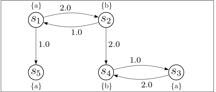
Example 3.5 Consider the example CT MC in figure 3.2 and the computation involved to check S≥0.3(b)for state s1. A graph analysis reveals that there are two
BSCCs in the example viz. B1 ={s3, s4} and B2 ={s5}.
s
1
{a}
s
2
{b}
s
3
{a}
s
4
{b}
s
5
{a}
2
.
0
1
.
0
1
.
0
2
.
0
2
.
0
1
.
0
Figure 3.2: BSCCs in Steady-State Analysis
The first step is to determine the set of states that satisfy b-formula. As s4
is the only b-state belonging to one of the BSCCs hence by the application of equation (3.2), the steady-state probabilityπ(s1, Sat(b)) is:
π(s1, Sat(b)) =
P(s1,♦B1)·πB1(s4)
,
where P(s1,♦B1) can be determined by a solution for:
P(s1,♦B1) =
2
3 ·P(s2,♦B1) and P(s2,♦B1) = 2 3+
1
3·P(s1,♦B1).
Hence P(s1,♦B1) = 74. For πB1(s4) the following equations have to be solved:
2·πB1(s3)−πB1(s4) = 0 and πB1(s3) +πB1(s4) = 1,
yielding πB1(s
3.8
Transient Measures
Given an MRM M= ((S,R, Label), ρ, ι), to resolve whether the transient prob-ability measure of the form s P p(ϕ) is satisfied by the given model and state s, it is first necessary to determine the probability with which the given path formula ϕ is satisfied. Define:
K(s) = {x∈I|ρ(s)·x∈J}, and K(s, s′) = {x∈I|(ρ(s)·x+ι(s, s′))∈J},
for closed intervals I and J. K(s) is an interval of time in I such that the state-rewards accumulated by being resident in state s for any length of time in K(s) is in J. K(s, s′) is an interval of time in I such that the sum of the
state-rewards accumulated by being resident in state s for any length of time in K(s, s′) and the impulse reward acquired by transition from state s to s′ is
in J. The probability density of moving from state s to s′ within x time-units
is P(s, s′, x) = P(s, s′)·E(s)·e−E(s)·x. Hence the probability of leaving state s within the interval I such that both the time and reward bounds are met after the outgoing transition has taken place is:
PJI(s) =
X
s′∈S
Z
K(s,s′)P(s, s
′)·E(s)·e−E(s)·x
dx, (3.3)
wheres, s′ ∈S. For instance consider the case where unbounded reward is allowed
to be accumulated:
P[0[0,,t∞])(s) = X s′∈S
Z t
0 P(s, s
′)·E(s)·e−E(s)·x
dx= X s′∈S
P(s, s′)·(−e−E(s)·x)
t 0 = X
s′∈S
P(s, s′)·(1−e−E(s)·t) = (1−e−E(s)·t)· X
s′∈S
P(s, s′) = (1−e−E(s)·t).
3.8.1
Ne
X
t Formula
For formula s P p(XJIΦ), let PM(s,XJIΦ) be the probability of satisfying the formula (XI
JΦ) starting from state s. From equation (3.3), PM(s,XJIΦ) is: PM(s,XI
JΦ) =
X
s′ Φ
P(s, s′)·(e−E(s)·inf(K(s,s′))
−e−E(s)·sup(K(s,s′))
). (3.4)
This characterization suggests that the algorithm to compute s P p(XJIΦ) proceeds by first obtaining all states that satisfy Φ. Subsequently, PM(s,XI
JΦ) is determined by the use of equation (3.4) and this probability is compared with the specified probabilityp. Special cases exist for the next formulas when J = [0,∞) and I = [0,∞):
PM(s,X[0[0,,∞∞))Φ) =PM(s,XΦ) = X s′ Φ
3.8. TRANSIENT MEASURES 27
3.8.2
U
ntil Formula
For formulasP p(ΦUJIΨ), letPM(s,ΦUJIΨ) be the probability of satisfying the formula (ΦUI
JΨ) starting from state s. For time-reward bounded until formula
P p(ΦUI
JΨ), PM(s,ΦUJIΨ) is characterized by a fixed-point equation. First let L⊖y = {l−y|l ∈ L∧l ≥ y}, then PM(s,ΦUI
JΨ) is the least solution of the following set of equations:
PM(s,ΦUI JΨ) =
1, ifs¬Φ∧Ψ and inf(I) = 0 and inf(J) = 0,
P
s′∈S
Rsup(K(s,s′))
0 P(s, s′, x)·PM(s′,ΦUJI⊖⊖x(ρ(s)·x+ι(s,s′))Ψ)dx, if sΦ∧¬Ψ, e−E(s)·inf(K(s))
+Ps′∈S
Rinf(K(s,s′))
0 P(s, s′, x)·PM(s′,ΦUJI⊖⊖x(ρ(s)·x+ι(s,s′))Ψ)dx, if sΦ∧Ψ, 0, otherwise.
(3.6)
The justification of this characterization is as follows:
1. s Ψ and inf(I) = 0 and inf(J) = 0: Since s satisfies Ψ and inf(I) = 0 and inf(J) = 0 then all paths starting from state s satisfy the formula and consequently the probability is 1.
2. sΦ∧¬Ψ: Ifs satisfies (Φ∧¬Ψ) then the probability of reaching a Ψ-state from state s within the intervalI and by accumulating reward r∈J is the probability of reaching a direct successors′ withinxtime-units, (x≤sup(I)
and (ρ(s)·x+ι(s, s′))≤sup(J), that isx≤sup(K(s, s′))) multiplied with
the probability of reaching a Ψ-state from states′ within the interval I⊖x
and by accumulating reward (r−(ρ(s)·x+ι(s, s′))).
3. sΦ∧Ψ: If ssatisfies (Φ∧Ψ) then the path formula is satisfied if the state s is not left for inf(K(s)) time-units. Alternatively, state s should be left before inf(K(s, s′)) time-units have elapsed in which case the probability is
defined as in case 2. Note that by definition inf(K(s, s′))≤inf(K(s)). Whilst the system of equations described above completely characterizes the until formula some trivial cases still exist. IfJ = [0,∞) and I = [0, t] for t∈R≥0
then the characterization of the path formula is given by the least solution of the following set of equations:
PM(s,ΦU[0[0,,t∞])Ψ) =
1, if sΨ,
Rt
0
P
s′∈SP(s, s′, x)·PM(s′,ΦU[0,t⊖x]Ψ)dx, if s Φ∧¬Ψ, 0, otherwise.
(3.7)
If J = [0,∞) and I = [0,∞) then:
PM(s,ΦU[0[0,,∞∞))Ψ) = PM(s,ΦUΨ). (3.8) The solution to the RHS of equation (3.8) is the least solution of the following set of linear equations:
PM(s,ΦUΨ) =
1, ifsΨ,
P
s′∈SP(s, s′)·PM(s′,ΦUΨ), if s Φ∧¬Ψ, 0, otherwise.
The solution to equation (3.8) can be computed by the solution of linear equations by standard means such as Gaussian elimination or iterative strategies such as the Gauss-Seidel method.
Example 3.6 Consider the WaveLAN modem model of example 3.1. In this ex-ample it is demonstrated as to how the value of the formulaPM(3, idleU[0,2]
[0,2000]busy)
can be computed using the characterization for until formula as presented in equa-tion (3.6).
By condition (2) in equation (3.6):
PM(3, idleU[0[0,,2000]2] busy) =
Z a
0 λIR·e
−E(3)·x·
PM(4, idleU[0[0,,20002−x]−1319·x−0.42545]busy)dx
+
Z b
0 λIT ·e
−E(3)·x·PM(5, idleU[0,2−x]
[0,2000−1319·x−0.36195]busy)dx,
where E(3) = (λIR+λIT +µIS), a= 20001319−0.42545, b = 2000−13190.36195. By condition (1) in equation (3.6):
PM(4, idleU[0[0,,20002−x]−1319·x−0.42545]busy) =PM(5, idleU[0[0,,20002−x]−1319·x−0.36195]busy) = 1,
hence:
PM(3, idleU[0[0,,2000]2] busy) =
Z a
0 λIR·e
−E(3)·xdx+Z b
0 λIT ·e
−E(3)·xdx
Assume rates λIR = 1.5 hr.−1, λIT = 0.75 hr.−1, µIS = 12 hr.−1, then:
PM(3, idleU[0,2]
[0,2000]busy) =
Z a
0 1.5·e
−14.25·xdx+Z b
0 0.75·e
−14.25·xdx = 0.10526 + 5.2632·10−2 = 0.15789.
Chapter 4
Model Checking MRMs
This chapter presents algorithms for model checking Markov Reward Models. An overview of the model checking procedure is provided in section 4.1. Section 4.2
describes algorithms for model checking steady-state formulas. In section 4.3, al-gorithms for model checking transient probability measures are described. Section
4.4presents numerical methods for model checking transient probability measures. Applications of the numerical methods for model checking transient probability measures are presented in section 4.5 and in section 4.6.
4.1
The Model Checking Procedure
For model checking MRMs, given a system modeled as an MRM and a formula expressed in CSRL, it has to be ascertained whether the formula is valid for the MRM. Initially the formula is parsed and its sub-formulas are determined. Then a post-order recursive traversal of the parse-tree is carried out to determine the values of the sub-formulas. The value of a formula is the set of states that satisfy the formula. Such a set of states that satisfy a formula Φ is referred to asSat(Φ). An algorithm to obtainSat(Φ) is algorithm 4.1.
Algorithm 4.1 SatisfyStateFormula
SatisfyStateFormula(StateFormula Φ): SetOfStates if Φ =tt then return S
if Φ∈AP then return {s|Φ∈Label(s)}
if Φ =¬Φ1 then returnS−SatisfyStateFormula(Φ1)
if Φ = Φ1 ∨Φ2 then return SatisfyStateFormula(Φ1) ∪ SatisfyStateFormula(Φ2)
if Φ =S p(Φ1) then return SatisfySteady(p,E,SatisfyStateFormula(Φ1))
if Φ =P p(XI
JΦ1)then return SatisfyNext(p,E,SatisfyStateFormula(Φ1), I, J)
if Φ =P p(Φ1UJIΦ2) then
return SatisfyUntil(p,E,SatisfyStateFormula(Φ1),SatisfyStateFormula(Φ2), I, J)
end SatisfyStateFormula
Algorithms to determineSatisfySteady, SatisfyNext andSatisfyUntil are presented in sections 4.2, 4.3.1 and 4.3.2 respectively.
4.2
Model Checking Steady-State Operator
The state formulaS p(Φ), given an MRMM= ((S,R, Label), ρ, ι) and a starting states∈S, asserts that the steady-state probability for the set of Φ-states meets the boundEp. As has been illustrated in chapter 3 when the underlying CTMC of Mis strongly connected then a standard CTMC steady-state analysis by the solution of a linear system of equations (3.1) suffices.
When the underlying CTMC ofMis not strongly connected then first a graph analysis is performed to determine all the bottom-strongly connected components (BSCCs). Every BSCC is a strongly connected component and standard CTMC analysis to determine the steady-state probability for each BSCC can be carried out. For finding maximal SCCs (MSCC) standard algorithms are available and can be readily modified to obtain BSCCs. To find BSCCs the Tarjan’s algorithm for obtaining MSCCs as presented in [Nuu93] is considered. Subsequently, every one of the MSCCs has to be further analyzed to determine if it is a BSCC. For this purpose it has to ascertained that all the successors of states belonging to a MSCC belong to the MSCC too.
Consider algorithm 4.2. The Tarjan’s algorithm has two procedures viz. pro-cedure visit and procedure getBSCC. Procedure getBSCC applies procedure visit
to all the states that have not been visited. Procedurevisit initially considers the state being visited as the root of a component. Subsequently all the successor states of the state being visited are considered. If one of the successor states is not visited yet then it is visited too. Once all the successor states have been visited the root of the state being visited is the minimum of its initial root and the roots of its successor states which are not already in a component. Note that minimum here refers to the dfs (depth-first search) order in which the states are visited. If at this point the root of the state being visited is still the original dfs order of the state then a MSCC is said to have been detected and the states in the MSCC are on the top of the stack.
With reference to the detection of the BSCC two cases arise during the evo-lution of the algorithm. When a certain state is being visited either it can transit to a state which has not been visited or to a state which has already been visited. If it can transit to a state that has already been visited either this new state is in the present stack or is part of a detected component and not in the stack. Consequently if a transition to a state already detected to be in a component is possible then the present component being detected can never be a BSCC. If a new state is visited then it would either be a part of the present component being detected or it would be a new component. If the new state is found to be in a new component then a transition to another component from the present state is possible. Consequently the component being visited can never be a BSCC.
4.2. MODEL CHECKING STEADY-STATE OPERATOR 31
The computational cost for Tarjan’s algorithm is O(M+N) time where M is the number of non-zero elements in the rate matrix andN is the number of states. The time-complexity of the modified Tarjan’s algorithm for detecting BSCC is
O(M +N) too.
Algorithm 4.2 Bottom-Strongly Connected Component getBSCC(StateSpace S, RateMatrix R): ListOfBSCC
initialize stack, bool [|S|] reachSCC, integer[|S|] root
initialize bool[|S|]inComponent, ListOfBSCCbscclist, integerdf sorder = 0
for each s∈S such that root[s] = 0
visit(s) /* root[s]=0⇒s is not visited */ end for
return bsccList
end getBSCC
visit(State s): void
increment df sorder
initialize integer remorder =df sorder
initialize BSCC newbscc, boolreachSCC =f alse
root[s] = df sorder, inComponent[s] =f alse,visited[s] =true
push(s, stack)
for each s′ ∈S such that R
s,s′ >0
if root[s′] = 0 then visit(s′)
if ¬inComponent[s′] then root[s] = min(root[s], root[s′])
else reachSCC[s] =true
end for
if root[s] = remorder then do
s′ =pop(stack)
reachSCC =reachSCC∨reachSCC[s′]
newbscc.add(s′)
inComponent[s′] =true
while s6=s′
if ¬reachSCC
then bscclist.add(newbscc) e