Non-Isotropic Length Scales During
the Compression Stroke of a Motored Piston Engine
STEPHAN BREUER1, MARTIN OBERLACK2and NORBERT PETERS3 1Delphi Automotive Systems, Technical Centre Luxembourg, Avenue de Luxembourg, L-4940 Bascharage, G. D. de Luxembourg
2Fachgebiet f¨ur Str¨omungsmechanik, Fachbereich f¨ur Mechanik, TU Darmstadt, Petersenstraße 13, 64287 Darmstadt, Germany; E-mail: [email protected]
3Institut f¨ur Technische Mechanik, RWTH Aachen, 52056 Aachen, Germany Received 25 July 2004; accepted 23 October 2004
Abstract. For the case of axial compression the two-point velocity correlation equations of ax-isymmetric homogeneous turbulence are derived. Appropriate integrations then lead to equations for the components of the Reynolds stress tensor as well as to those for the two independent integral length-scales characterizing axisymmetric homogeneous turbulence. These equations contain a cer-tain number of empirical constants. Values for these constants are taken from the literature, or were adjusted from the present data.
The resulting model is validated using data from a motored piston engine. The flow field, which has negligible swirl and tumble, has been measured using particle image velocimetry (PIV). Since turbulence is axisymmetric and homogeneous in the counter region, two-dimensional PIV provides the time history of the axial and radial length-scales. The experimental data are compared with the mathematical model.
Key words: compressed turbulence, two-point correlation, non-isotropic turbulence, length scale equation, piston engine, compression stroke, PIV
1. Introduction
In many turbulent flows of practical interest the assumption of a single integral length-scale or corresponding assumptions of a scalar dissipation rate is not appro-priate [1]. This is particulary true for flows with one preferred direction. Under the absence of a mean velocity gradient we may consider the theory of homogeneous turbulence or the specific case of axisymmetric homogeneous turbulence, which describes the evolution of a multi-point correlation tensor in axisymmetric form or in the case of a single-point approach two independent turbulence intensities and two independent turbulent length-scales. Axisymmetric turbulence is a natural extension of isotropic turbulence which accounts for the anisotropic character of the turbulence parameters.
compression and anisotropy perpendicular to it we need at least two length-scales and two turbulence intensities to describe the turbulent flow adequately.
In the present paper we model the turbulence dynamics of a compression stroke by employing the simplification of the axisymmetric turbulence extended by one-dimensional homogeneous compression using two-point correlations. The theory of axisymmetric turbulence traces back to the work by Batchelor [2] and Chandrasekhar [3] who laid the foundation of this theory. Lindborg [4] recasted the theory in a different form, in which he introduced expressions based on cylindrical coordinates that can be directly validated experimentally.
On the basis of the latter approach the theory of axisymmetric turbulence will be extended to the case of axisymmetric compression in the present paper. Equa-tions will be presented for the corresponding two-point velocity correlaEqua-tions. In addition, following the procedure introduced in Oberlack [1] a modelling approach is developed to derive a closed set of equations for both the turbulence intensities and the integral length-scale in tensorial form.
The model for the compression of axisymmetric homogeneous turbulence pre-sented in this paper will be validated by measurements. The compression of turbu-lence is performed in a piston engine with a pancake chamber. In the literature the determination of turbulent length-scales and turbulence intensities in a piston en-gine using laser doppler velocimetry (LDV) have been detailed by H¨uppelsh¨auser [5], Hong and Tarng [6], and Lorenz and Prescher [7] to name only a few. In order to determine turbulent length-scales the LDV technique is applied simultaneously at two points in space. By varying the distance of the two points and after conducting a statistical analysis, the two-point velocity correlation may be determined along a given line. In all the above references the theory of isotropic turbulence has been employed to determine length-scales from the velocity correlation data. Since the theory of isotropic turbulence was used, non-isotropic length-scales could not be obtained.
In this paper particle image velocimetry (PIV) will be applied to determine the flow field and other quantities to be derived thereof. PIV is a two dimensional, nonintrusive optical measuring technique. It was developed at the beginning of the [8, 9], and since then has been continuously improved to become a standard measuring technique, which also has been applied to velocity field measurements in engines (see e.g. [10, 11] 1980s). Since PIV yields a two dimensional field of data, a two dimensional correlation function may be calculated under the assumption of a homogeneous axisymmetric turbulence statistic. In turn this may be used to compute statistical quantities such as turbulent length- and velocity scales to verify turbulence model equations.
2. Two-Point Correlation Equations
in particular the compression velocity. Employing this asymptotic assumption we obtain the well known zero-Mach number limit of the Navier-Stokes equations where density ρ is only a function of time. As an immediate consequence the temporal density variations act as a source term in the mean continuity equation
∂u¯k
In order to derive a model for the compression of axisymmetric homogeneous turbulence the concept of two-point correlation will be introduced. Following Rotta [12] the two-point correlation is defined as
Ri j(x,r,t) = u′ i(x,t)u
′
j(x+r,t). (2)
In the limit of zero separation r the two-point correlation Ri j converges to the
Reynolds stress tensoru′ iu
′
j. In addition to the two point correlation we define the
triple correlation as
R(i k)j(x,r,t) = u′i(x,t)u′k(x,t)u′kj(x+r,t),
Ri(j k)(x,r,t) = u′i(x,t)u′j(x+r,t)uk′(x+r,t), (3)
which obeys the intercorrelation
R(i k)j(x,r,t)= Rj(i k)(x+r,−r,t). (4)
Furthermore a two-point pressure-velocity correlation is introduced, which is de-fined as
with the corresponding relation
p′u′
i(x,r,t)=u ′
ip′(x+r,−r,t). (6)
Using these definitions a general transport equation for the two-point correlation
Ri j may be derived. For the case of homogeneous turbulence all correlations are independent of the locationx. The transport equation forRi jmay be simplified and
yields
∂xj is at most a function of time and the last term in the first line simplifies to−rl∂u¯k
∂xl ∂Ri j
Taking the divergence of Equation (7) yields a Poisson equation foru′ ip′
1 ρ
∂2p′u′ j
∂rk∂rk =2
∂uk¯ ∂xl
∂Rl j
∂rk −
∂2R(kl)j
∂rk∂rl . (8)
The two-point correlation, the triple correlation and the two-point pressure-velocity correlation have to satisfy additional constraints derived from the continuity equation
∂Ri j
∂ri =0,
∂Ri j
∂rj
=0, ∂R(i k)j ∂rj
=0, ∂R(i k)j ∂rj
=0, ∂u
′ jp′
∂rj =0
and ∂p
′u′ i
∂ri =0. (9)
In case of homogeneous turbulence the Equations (4) and (6) reduce to
Rj(i k)(r)= −R(i k)j(r) u′jp ′(
r)= −p′u′
j(r). (10)
2.1. EQUATIONS FOR AXISYMMETRIC TURBULENCE
Homogeneous axisymmetric turbulence is a special case of homogeneous turbu-lence and is defined by one preferred direction λ. All statistical properties are
invariant with regard to translation in space, finite rotation and mirroring of the coordinate system aboutλ. This implies that all tensors in Equation (7) have to be
written as axisymmetric tensors. All tensors depend on a correlation separationz
in the direction of theλ-axis and a separationlperpendicular toλ.
In order to obtain a set of scalar equations for axisymmetric turbulence, all tensors are transferred into a cylindrical coordinate system, in which thez-axis is parallel to the significant directionλ.
This idea was first introduced in [4] since it considerably simplifies both classical notation from [2, 3] as well as its comparison to measurable quantities. In the present and the following Section 2.2 this extension of the classical work and the ideas of [4] are further extended to compressed turbulence i.e. slow compression (zero Mach number limit) either inz- orr-direction.
According to the theory of invariants a second order axisymmetric tensor may be written as (see e.g. [2, 3])
Ri j(λ,r)= A(l,z)rirj+B(l,z)δi j+C(l,z)λiλj+D(l,z)(λirj+λjri). (11)
In Equation (11)ri is the component of the correlation vector to an arbitrary location in space while λi is the component of the unity-vector parallel to thez
tensor Ri j may be reduced to two independent components (see [2])
Following [3] the axisymmetric vector for the pressure-velocity correlation may be written as
Pi(r)= p′u′
i(r)=M(l,z)ri+N(l,z)λi. (14)
Rewriting the latter in a cylindrical coordinate system one obtains two distinct com-ponents of the pressure-velocity correlation which are interrelated by the continuity Equation (9) according to
0= ∂(l
The same decomposition as in (11) and (14) may be applied to the third order tensor, which may according to [3] be written as
R(i k)j(r)=F(l,z)rirjrk +G(l,z)λiλjλk
+H1(l,z)rirjλk+H2(l,z)[rirkλj+rjrkλi]
+I1(l,z)[rjλiλk+riλjλk]+I2(l,z)rkλiλj
+J1(l,z)[riδj k+rjδi k]+J2(l,z)δi jrk
+K1(l,z)[λiδj k+λjδi k]+K2(l,z)δi jλk (16)
After transforming the latter into a cylindrical coordinate system we obtain ten distinct components of the tensor. These components are interrelated to each other by the equation of continuity (9) according to
0=∂
As a result, six independent components of the triple correlation tensor remain.
Note that in the limit of zero separationl → 0 andz → 0 the triple correlations
2.2. DYNAMIC EQUATIONS FOR AXISYMMETRIC COMPRESSED TURBULENCE
In order to derive equations for homogeneous axisymmetric turbulence, the vectors and tensors in Equation (7) have to be replaced by axisymmetric tensors and the entire equation has to be transformed into a cylindrical coordinate system. From the continuity Equation (13) we learn that only two independent scalar equations remain.
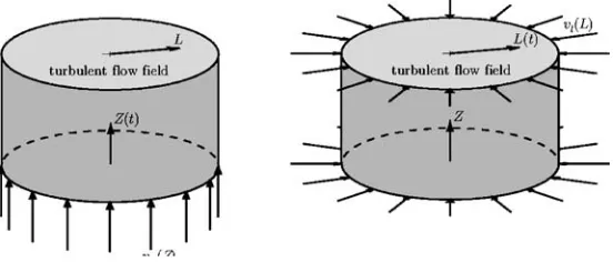
A special treatment for the compression term has to be taken into account. In case of axisymmetric homogeneous turbulence two cases of compression need to be distinguished: compression in direction of the axis of symmetry (Figure 1 left) and compression perpendicular to the axis of symmetry (Figure 1 right). Within this paper only the compression in the direction of the axis of symmetry is considered, because of the direction of a compression stroke in a piston engine.
The mean velocity fields for the cases in Figure 1 are derived from the equation of continuity
∂u¯z(Z,t)
∂Z = −
1 ρ
∂ρ ∂t ≡
1
h0(t)
dh0(t)
dt and
1
L
∂Lu¯l(L,t)
∂L
= −
1 ρ
∂ρ ∂t ≡
2
r0(t)
dr0(t)
dt , (18)
where h0(t) andr0(t) respectively denote the time-dependent cylinder hight and
radius. Note thatZandLmay not be confused withzandl.Z andLare the physical coordinates whilezandldenote correlation space variables.
Integrating (18) we respectively obtain
¯
uz(Z,t)=Z
1
h0(t)
dh0(t)
dt and u¯l(L,t)=L
1
r0(t)
dr0(t)
dt . (19)
Using these expressions for the compression term in (7), the explicit dependence on the physical coordinatesLandZvanishes and the entire equation only depends on the correlation space variableslandz.
For the case of compression in axial direction the transformation of Equation (7) to cylindrical coordinates respectively yields the correlation equation in axial di-rection and the cross-correlation equation
∂Rll
For the subsequent analysis it may be useful to employ the equation for the cor-relation in axial direction Rzz, which can be derived from the equation of the cross-correlation (21) together with the equation of continuity (14) leading to
∂Rzz
Transformation of the Poisson equation for the pressure yields one equation for the pressure-velocity correlation for the case of axisymmetric turbulence. Interestingly enough the resulting equation may be integrated once with respect tozby employing continuity equations for the pressure-velocity (15) and for the triple-correlation (17)
1
The similar procedure as above may be applied to derive a set of equations for isotropic turbulence under spherical compression. In this case only one equation for the longitudinal two-point correlation remains (see [13])
∂Rrr
whereris the spherical correlation coordinate. The latter equation is an extended version of the classical von-K´arm´an-Howarth equation for incompressible isotropic turbulence (see [14]). The Poisson equation for the pressure-velocity correlation vanishes identically in this case.
Introducing the scaling transformation
˜
into Equation (23) the compression term can be eliminated and the classical form of the von-K´arm´an-Howarth equation is recovered
∂R˜rr(˜r,˜t)
with the only difference that viscosity has become a time-dependent quantity. It is important to note that for the case of homogeneous axisymmetric turbulence no such transformation exists, which eliminates the compression terms. This is because the prefactors of the compression terms in Equations (20)–(22) are different as has been mentioned above. Hence compression is an essential non-trivial property of the equations of axisymmetric turbulence.
3. One-Point Equations for Compressed Homogeneous Axisymmetric Turbulence
The set of equations for the two-point correlations may be used to derive equations for the Reynolds-stress tensor, the dissipation tensor or alternatively the length-scale tensor. As in the previous section we consider homogeneous turbulence and hence all dependencies on the locationxvanish.
The two-point correlation Ri j converges to the Reynolds-stress tensor in the
limit of zero separationr
from which we define the turbulent kinetic energy according tok = 1 2u
′
mu′m. Cor-respondingly the dissipation tensor may be derived from the two point correlation tensor as (see [15])
εi j(t)=lim
from which we obtain the scalar dissipation rate
ε=εkk. (28)
From the two point correlation tensor we may also define the integral length-scale tensor (see e.g. [16])
i j(t)=
from which immediately leads to a scalar integral length-scale
(t)=mm(t). (30)
Since the explicit functional form of Ri j is unknown, [15] employed the Cayley-Hamilton theorem in order to model a relation between the integral length-scale tensor, the dissipation tensor and the Reynolds-stress tensor according to
i j =
where the tensorsbi j anddi j are respectively the anisotropy part of the Reynolds-stress and the dissipation tensor defined by
bi j =
The coefficientsϕ(m,n)may depend on the scalar tensor invariants ofbi janddi j(see [15]). For the model to be presented here,i j is assumed to be a linear function of bi j and di j. In the following subsection equations for the components of the Reynolds-stress tensor and the length scale tensor will be presented for the case of compressed homogeneous axisymmetric turbulence.
3.1. MODELLING THE ONE-POINT EQUATIONS FOR AXISYMMETRIC COMPRESSED TURBULENCE
Introducing the limits l → 0 and z → 0 into Equations (20)–(22) we obtain
the Reynolds stress equation for homogeneous axisymmetric compressed turbu-lence. Only the trace elements of theu′
iu ′
j tensor remain, which for axisymmetric
turbulence only constitute two independent componentsu′2
z andu ′2
subsequently. Thus, two scalar equations are sufficient to describe the Reynolds-stress tensor in case of axisymmetric turbulence. The turbulence energy is given by
k = 1
2u
′2
z +u′l2. (33)
The integration of the Equations (20)–(22) according to the definition of the integral length-scale (29) yields scalar equations for the components of the length-scale tensor. As in the case of the Reynolds-stress tensor, only two independent elements
in the trace of the length-scale tensor remain as well. A scalar length-scale is
defined by the trace of the length-scale tensor
=zz+2ll. (34)
The detailed derivation beginning from the two-point correlation to the Reynolds-stress tensor and to the length-scale tensor is pointed out in [1, 15]. Applying the one-point limit to Equations (20)–(22) extended by a model for the dissipation and redistribution leads to
du′2
Combining Equations (35) and (36) according to Equation (33) we derive an equa-tion for the turbulent kinetic energy
dk
The equations for the components of the length-scale tensor are
Combining Equations (38) and (39) according to Equation (34) we obtain an equa-tion for the turbulent kinetic energy
d
The model parameters are according to [15, 17]
c=0.1643 a0=0.05 cR =4 cεR =0.8 and cε2=1.92.
As is explained in the appendix, the parametersa1anda3are set to zero.
Equations (35)–(40) form a complete set of one-point equations to model com-pressed homogeneous axisymmetric turbulence. In contrast to the case of isotropic turbulence, no analytical solution of this set of equations may be derived.
3.2. APPLICATION OF THE TURBULENCE MODEL TO THE COMPRESSION
OF TURBULENCE IN A PISTON ENGINE
The compression terms in Equations (35)–(40) are expressed by the motion of a piston in an engine according to
d lnh0(t)
whereω,α,ǫandλare respectively rotational engine speed, crane angle, compres-sion ratio and crank shaft ratio.
Introducing this equation implies that the top dead center (TDC) before the com-pression stroke is equal to 0◦cranc angle (CA) and that the TDC of the compression
stroke is equal to 180◦CA.
The engine, which has been employed to validate the theoretical results in Chapter 4 possesses a crank shaft ratio λ = 0.29 and a compression ratio of ǫ =8.5.
In order to solve the set of Equations (35)–(40), dimensionless variables have to be introduced, which define the state of turbulence at the beginning of the com-pression. Combining the initial conditions for the turbulence energy, the scalar length-scale and the engine speed, we obtain the dimensionless variableσ, which is defined as
the time scale of turbulence. In addition toσtwo values are required as initial condi-tions, which contain the degree of Reynolds-stress and length-scale anisotropy at the beginning of the compression. As the appropriate characteristic variables we define
γ =
u′2
l0
u′2
z0
and δ= ll0
zz0
. (43)
Isotropy means that both ratios, i.e. the Reynolds-stress tensor anisotropyγ as well as the length-scale stress tensor anisotropyδ, are equal to 1. For the subsequent anal-ysis we assume the same degree of anisotropy for both the Reynolds-stress tensor and the length-scale tensor at the beginning of the compression and henceδ=γ.
4. Experimental Model Verification
The aim of the experimental investigations is the validation of the one-point model equations in Section 3 of the compression of homogeneous axisymmetric turbu-lence. Homogeneous axisymmetric turbulence is realized by the compression of air in a combustion chamber of a four stroke piston engine at the absence of combus-tion. It is important to note that there were also no tumble or swirl in the flow. In order to derive the components of the Reynolds-stress and the length-scale tensor, the fluid velocity within the chamber has to be determined. For this purpose we ap-plied the particle image velocimetry (PIV) technique, which is a two dimensional, non-intrusive, optical technique for instantaneous velocity measurement. Since we have axisymmetric turbulence, the mean velocity and the statistical quantities are entirely described by two-dimensional information.
4.1. EXPERIMENTAL DEVICE
Measurements were conducted in a 1.6 L four cylinder transparent engine from Volkswagen company, which is based on the 827 series. Optical access to the combustion chamber was given by quartz windows (size: 20 mm × 20 mm) in
the upper part of an intermediate housing between the cylinder head and the cranc casing. For each cylinder two windows were mounted opposite each other. The two outer cylinders contain a third window, which is arranged perpendicular to the two other windows.
The transparent engine is characterized by the data in Table I (see [18, 19]). The engine has been motored by a dynamometer without fuel and combustion.
4.2. PARTICLE IMAGE VELOCIMETRY
Table I.Characteristic engine parameters.
Number of cylinders 4
Bore 79.5 mm
Stroke 80 mm
Compression ratio 8.5:1
Cranc shaft ratio 0.29
Maximum engine speed 4000 rpm
Shape of combustion chamber disc-shaped
particle size decreases. The measuring plane is defined by a thin two dimensional light sheet located parallel to the combustion chamber axis. The particles, which are moving in the light sheet plane, induce an optical signal, which is recorded in perpendicular direction by a camera. By using a pulsed light source, multiple images of the individual particles moving in the light sheet plane are recorded on the same photographic film. With the knowledge of the time difference between pulses the separation of the particle images on the film yields a two dimensional velocity vector. Using a high speed camera, these multiple images can be recorded on separated frames.
The intake flow of the engine was seeded with a mixture of TiO2 and SiO2
particles which have a size of approximately 10µm. A copper vapor laser ACL25 from OXFORD-LASERS was used to create the light sheet. The laser frequency can be selected between 8 and 32 kHz. At a nominal frequency of 10 kHz the pulse energy is approximatively 4 mJ with a pulse length between 15 and 60 ns. The wavelength of the emitted light is 510 and 577 nm. A laser con-troller, which was triggered externally by a camshaft signal, synchronizes laser pulses, camera and engine. A CORDIN drum camera was used to capture the images. With a film length of 1 m, 50 images with a size of 24 mm×18 mm
were recorded. For the results presented below a laser frequency of 15 kHz was adopted.
The measuring plane was located just below the cylinder head between the inlet valve and the exhaust valve. The laser light is coupled in and out by the two quartz windows in opposite position. The height of the measuring plane is limited by the size of the windows, which is 20 mm×20 mm. Since the measurements were
performed in the first cylinder, the scattered light was recorded through a third win-dow, which was installed perpendicular to the light sheet. The experimental setup of the camera, the light sheet and the compression volume are shown in Figure 2.
The markers, which are shown in Figure 2 are used to define a fixed coordinate system for each image frame. They were recorded on each image and enable a perfect alignment of subsequent images to each other.
Figure 2. Set up and measuring plane in the combustion chamber.
[20]. The cross-correlation function of two subsequent images is defined by:
Corr(x, y)=
∞
−∞
∞
−∞
g(x,y)h(x −x,y−y)d yd x. (44)
This operation is performed on small subimages of digitized PIV-images, which yields a displacement vector for each subimage. This displacement vector is defined by the absolute maximum of the correlation function. For the PIV-evaluation per-formed within this paper also the second and the third maximum was determined. A post-processing operation selects the displacement of the three maxima, whose vector fits best to the entire vector field with respect to the neighboring vector field. The best choice of such a vector is calculated from the neighboring vectors assuming solid body rotation (45)
uA =uP +ω×rA P, (45)
whereuP,ω,rA P anduA are respectively the velocity vector, the rotation vector,
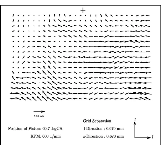
the distance vector between the given and the remote point and the velocity at the remote point, whereto the velocity is extrapolated. An example of a post-processed velocity field is shown in Figure 3.
4.3. ANALYSIS OF THE VELOCITY DATA
Figure 3. Example of an instantaneous velocity field from PIV measurement.
The difference between the mean velocity field and the instantaneous velocity field
yields the field of the velocity fluctuations u′
i. These fluctuations were used to
calculate the stress tensor and the length-scale tensor. The Reynolds-stress tensoruiuj was calculated with
uiuj =
1
M·N
i
j
u′ iu
′
j, (46)
whereiandjare the indices denoting the directionszandlof the flow field.
With the assumption of axisymmetric turbulence all components of the Reynolds-stress tensor were calculated using Equation (46). From the latter formula and together with the definition of the turbulent kinetic energy and (33) we obtain
k =v′ lv
′ l +
1 2v
′
zvz′, (47)
The length-scale is obtained from the cross- or auto-correlation function of the velocity field, which is defined by:
Ri j(l,z)=
1
(m−l)·(N−z)
˜
l
˜
z
u′i(˜l,˜z)u′j(˜l+l·˜l,z˜+z·z˜) (48)
wherez˜ and˜ldenote the grid spacing inz- andl-directions respectively.
we obtain
i j =
3 4 1 k
∞
z=−∞
∞
l=∞
Ri j(l,z)
l
l2+z2dld z, (49)
which in decretized form reads
i j =
3 8
zl k
b−1
˜ j=−(b−1)
a−1
˜ i=0
(2˜i+1)l
(2˜i+1)2l2+(2 ˜j+1)2z2Fi j(l˜i,l˜i+1,z˜j,z˜j+1)
(50)
with
Fi j(l˜i,l˜i+1,z˜j,z˜j+1)= fi j(li˜,z˜j)+ fi j(li˜,z˜j+1)+ fi j(l˜i+1,z˜j)+ fi j(l˜i+1,z˜j+1).
(51)
The length-scale tensor for homogeneous axisymmetric turbulence as well as the Reynolds-stress tensor contain only values in the main diagonal. The trace of the length-scale tensor yields the scalar length-scale
=2·ll+zz. (52)
Calculating the length-scale by using the approach presented here requires the assumption of homogeneous axisymmetric turbulence. This assumption is consid-erably weaker than the assumption of isotropic turbulence, which is usually adopted to calculate a turbulent length-scale from one or zero dimensional velocity fields, obtained from LDV measurements [5, 7].
5. Results
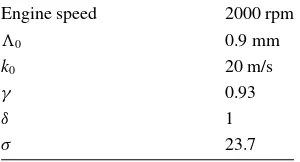
The model of homogeneous axisymmetric compressed turbulence was validated against the experimental data taken from a piston engine as described in Section 4. The boundary conditions at the beginning of compression, which are required for the mathematical model, are obtained from the experimental data (see Table II).
Table II.Initial conditions for the calcu-lation of axisymmetric turbulence.
Engine speed 2000 rpm
0 0.9 mm
k0 20 m/s
γ 0.93
δ 1
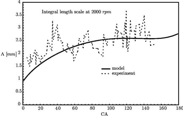
Since the main interest is focused on the development of the turbulent length-scale, only the length-scale data is considered within this paper. Since the nor-malized length-scale is independent of the engine speed only the results of the length-scale at 2000 rpm are presented within this paper.
Experiment and model agree reasonably well as will be demonstrated in the
subsequent figures. The integral length-scale in Figure 4 increases during the
compression stroke. The minimum slope is observed between 120◦ CA and 150◦
CA and not at the end of the compression phase. The model reveals that, depending on the initial conditions and the strength of the compression the slope may change its sign during the compression stroke. This means that for a certain time interval during the compression stroke, the integral length-scale decreases.
A similar behaviour is observed for the two individual components of the
length-scale tensor. The length-scale in radial directionll in Figure 5 increases
at the beginning and at the end of the compression phase, while between 90◦
CA and 150◦ CA a weak decrease of the length-scale is noticed. A continuous
increase of the length-scale is noted in the direction of the compression in Fig-ure 6. This is in contrast to the decrease of the combustion chamber height. The result of the model equation, which predicts that all elements beside the trace elements of the length-scale tensor disappear, is confirmed by the experimental data.
The varying behaviour of the length scale evolution such as an increase or decrease may be interpreted in the light of two main effects in Equation (40). At the absence of compression the integral length scale always increases due to the last term which always acts as a source term with the model constants given below (40).
Figure 5. Comparison of experimental data with the calculations of the radial component of the integral length-scalerrat 2000 rpm.
Figure 6. Comparison of experimental data with the calculations of the radial component of
the integral length-scalezzat 2000 rpm.
Only the compression term, the first term on the right hand side of (40) may decrease
. Since the term in square brackets is usually positive,d ln(h0(t))
Figure 7. Model calculation of the Reynolds-stress and the length-scale tensor for 1000 rpm with almost isotropic initial conditions.
Although there is a difference between the exact values of the model and those of the experimental data, the tendencies of both agree quite well with each other. This means that the model, which has been derived, describes the tendency of the length-scale evolution quite well for the compression of homogeneous axisymmet-ric turbulence. The difference between the theoretical and experimental values are twofold. First the experimental data still exhibits a certain amount of scatter, though several hundred samples have been taken. Second the validity of the assumption of homogeneous axisymmetric turbulence in the combustion chamber of the engine during the compression stroke is not fully valid. Though flow visualizations made it very clear that there is no swirl and tumble in the flow, inlet- and wall-effects decrease the validity of the underlying assumption.
In addition to the latter results the model for homogeneous axisymmetric tur-bulence yields information on if and when turtur-bulence becomes isotropic. For the present model isotropic turbulence means that the two components of both the length-scale and the Reynolds-stress tensor are equal to each other. The result presented in Figure 7 reveals that isotropic turbulence is essentially non-existing particularly during the late stage of compression. This result is independent of isotropic or anisotropic initial conditions as can be taken from Figure 7 where both Reynolds-stress and length-scale tensors have been chosen to be isotropic atα =0.
6. Summary
by [2, 3] were extended to include weak compression in the zero Mach number limit. The theory was written in cylinder coordinates as has been suggested by Lindborg [4]. In contrast to isotropic turbulence where spherical compression may be eliminated from the dynamic equation, the von-K´arm´an-Howarth equation, by a simple scaling transformation, the same is not true for unidirectional compression of homogeneous axisymmetric turbulence. As a result compression is an essential non-trivial part of the new theory which was not even implicitly included in the classical theories.
In addition to the two-point approach the two-tensor one-point model by Oberlack [1] was adopted and extended for the description of the compression of axisymmetric turbulence. This model was validated by experimental data from a four stroke piston engine at the absence of combustion. Axisymmetric turbulence is a good approximation of the flow in the latter device. From the model equation it was shown that exactly two independent length-scales exist, one in axial direction and another in radial direction. Both length-scales may be combined to the usual scalar integral length-scale.
In case of isotropic turbulence only one integral length-scale and the tur-bulent kinetic energy are sufficient to characterize turbulence in the one-point limit. Homogeneous axisymmetric turbulence turns into isotropic turbulence, when both the length-scales and Reynolds-stresses in radial and axial direction be-come equal. The one-point model reveals that isotropic turbulence exists in the case of compression of axisymmetric turbulence only as a transient state at the very beginning of the expansion phase, if the initial conditions were chosen isotropic.
For an experimental validation of the one-point model the PIV technique was applied to obtain velocity data from a turbulent flow field under homogeneous axisymmetric compression. A procedure to analyze two-dimensional turbulence data was presented, which yields two independent length-scales for homogeneous axisymmetric turbulence.
There are essentially two mechanisms that determine the behaviour of the length-scale evolution i.e. an increase or decrease of the integral length-length-scale. At the absence of compression the integral length scale always increases regardless of whether isotropic or axisymmetric turbulence is considered. This well known effect is properly modelled even with simple two-equation models. Only the compression term, which is present in both the two- and the one-point equations may decrease. Whether an increase or a decrease is observed depends on the sign of d ln(ho(t))
dt , the
temporal change of the logarithm of the cylinder hight. For the case of compression the latter term is always negative and hence the difference between the sink and the source term determines an increase or decrease of the integral length-scale. In case of an expansiond ln(ho(t))
dt is always positive and hence the integral length-scale always
7. Discussion on the Model Parametersa1anda3
The parametersa1anda3are related by the simple expression
a1=const1
a3
const2+a3
, (53)
and hence we finda1=0 ifa3=0 (see e.g. [1]).
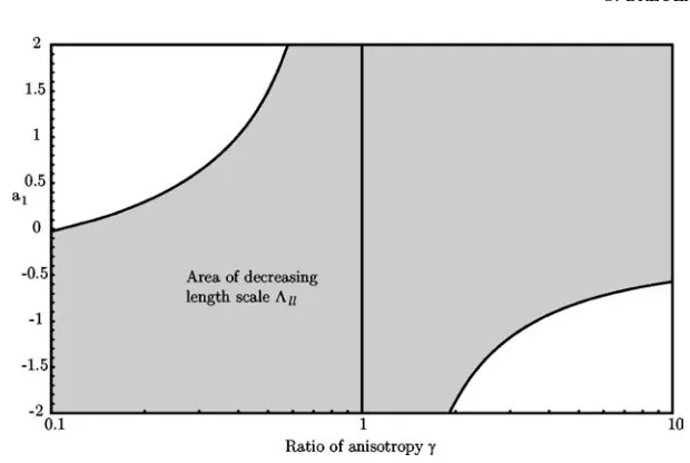
Figure 8. Combination of parametera1and coefficient of anisotropyγfor beginning of com-pression, which yields a negative sign for the change of the scalar length-scaleat the start of compression.
Figure 10. Combination of parametera1 and coefficient of anisotropy γ for beginning of
compression, which yields a negative sign for the change of the scalar length-scalellat the start of compression.
In the following a discussion on the parametera1is given for the case of rapid compression. Therefore the length-scale Equations (38)–(40) are analyzed by ne-glecting the dissipation of the length-scale terms. In this limit we investigate the sign of the compression term depending on the length-scale and the parametera1. For the two components of length-scale tensorll andzz and for the scalar length-scale the Diagrams (8)–(10) show the combination of the parametera1 versus the coefficient of anisotropyγ, for which the individual length-scale de-creases. The borderlines between the area of a positive sign and the area of negative sign are described by Equations (54)–(56):
equation for: a1
equation forzz: a1
References
1. Oberlack, M., Non-isotropic dissipation in non-homogeneous turbulence,J. Fluid Mech.350 (1997) 351–374.
2. Batchelor, G.K., The theory of axisymmetric turbulence,Proc. Roy. Soc.A 186(1946) 480–502. 3. Chandrasekhar, S., The theory of axisymmetric turbulence,Phil. Trans. Roy. Soc.A 242(1950)
557–577.
4. Lindborg, E., Kinematics of homogeneous axisymmetric turbulence,J. Fluid Mech.302(1995) 179–201.
5. H¨uppelsh¨auser, Experimentelle Untersuchung der Str¨omung und des W¨arme¨ubergangs im Kol-benmotor.PhD thesis at RWTH-Aachen, VDI Dusseldorf (1992).
6. Hong, C.W. and Tarng, S.D., Direct measurement and computational analysis of turbulence length scales of a motored engine,Experimental Thermal and Fluid Science16(1998) 277– 285.
7. Lorenz, M. and Prescher, K., Cycle Resolved LDV Measurements on a Fired SI-Engine at High Data Rates Using a Conventional Modular LDV–System.SAE900054(1990).
8. Adrian, R.J., Developement of Pulsed Laser Velocimetry for measurement of Fluid Flow.8th Biennial Symposium on TurbulenceUniversity of Missouri–Rolla (1984).
9. Meynard, R., Instantaneous velocity field measurements in unsteady gas flow by speckle ve-locimetry,Applied Optics22(1983) 535–540.
10. Reuss, D.L., Adrian, R.J., Landreth, C.C., French, D.T. and Fansler, T.D., Instantaneous Planar Measurements of Velocity and Large-Scale Vorticity and Strain Rate in an Engine Using Particle-Image Velocimetry.SAE890616(1989).
11. Rouland, E., Trinite, M., Dionnet, F., Floch, A. and Ahmed, A., Particle Image Velocimetry Measurements in a High Tumble Engine for In-Cylinder Flow Structure Analysis.SAE972831 (1997).
12. Rotta, J.C.,Turbulente Str¨omungen. B.G. Teubner Stuttgart (1972).
13. Breuer, S., Experimentelle und theoretische Untersuchung achsensymmetrischer Turbulenz w¨ahrend der Kompressionsphase in einer Kolbenmaschine.PhD thesis at the RWTH-Aachen, Couvellier Verlag G¨ottingen (2000).
14. de K´arm´an, T. and Howarth, L., On the statistical theory of isotropic turbulence,Proc. Roy. Soc. A 164(1938) 192–215.
15. Oberlack, M., Herleitung und L¨osung einer L¨angenmaß- und Dissipations-Tensorgleichung f¨ur turbulente Str¨omungen.PhD thesis, RWTH-Aachen, VDI D¨usseldorf (1994).
16. Sandri, G. and Cerasoli, C., Fundamental research in turbulent modeling,ARAP Rep.438(1981). 17. Jischa, M., Konvektiver Impuls-, W¨arme und Stoffaustausch. Vieweg-Verlag Braunschweig/
Wiesbaden (1982).
18. Holtorf, J., Messung zweidimensionaler Geschwindigkeitsfelder am Beispiel einer Motorinnen-str¨omung.PhD thesis at RWTH-Aachen, VDI D¨usseldorf (1992).
19. Wirth, M., Die turbulente Flammenausbreitung im Ottomotor und ihre charakteristischen L¨angenskalen.PhD thesis at the RWTH-Aachen, VDI D¨usseldorf (1993).