The journal homepage www.jpacr.ub.ac.id p-ISSN : 2302 – 4690 | e-ISSN : 2541 – 0733
Vibrational Resonance in the Classical Morse Oscillator Driven by
Narrow-Band and Wide-Band Frequency Modulated Signals
S.Guruparan1, B. Ravindran Durai Nayagam2, V. Ravichandran3, V. Chinnathambi3,* and S. Rajasekar4,!
1
Department of Chemistry, Sri K.G.S. Arts College, Srivaikuntam-628 619, Tamilnadu, India.
2 Department of Chemistry, Pope’s College, Sawyerpuram
-628 251,Tamilnadu, India.
3
Department of Physics, Sri K.G.S. Arts College, Srivaikuntam-628 619, Tamilnadu, India.
4
School of Physics, Bharathidasan University, Thiruchirapalli-620 024, Tamilnadu, India.
*
Corresponding email : [email protected]
!
Received 6 June 2016; Revised 20 August 2016; Accepted 21 September 2016
ABSTRACT
The phenomenon of vibrational resonance (VR) in the classical Morse oscillator influenced by narrow band and wide band, frequency modulated signals is numerically studied. Vibrational resonance was found to occur when the amplitudes f and g and
frequencies ω and Ω of the signals were varied. The dynamics of the system is studied
in the presence of both signals separately. Vibrational resonance and dynamics of the system were characterized using the response amplitude and bifurcation diagram.
Key word: Vibrational resonance, Classical Morse oscillator, Narrow-band frequency modulated signal, Wide- band frequency modulated signal, Response amplitude.
1. INTRODUCTION
The phenomenon of vibrational resonance (VR) in which the response of the system to a weak periodic signal can be enhanced by the application of the high-frequency periodic perturbation of appropriate amplitude. The analysis of VR has received a considerable interest in recent years because of its importance in a wide variety of contexts in science and engineering. For example, Landa and Mc Clintock [1] have shown that the occurrence of resonant behaviour with respect to a low-frequency force caused by the high-frequency force in a bistable system and later Gitterman [2] proposed an analytical treatment for this resonance phenomenon. Experimental evidence of the vibrational resonance has been demonstrated in analog simulations of the overdamped duffing oscillator [3], in an excitable
electronic circuit with Chua’s diode [4] and in a bistable optical cavity laser [5]. It has been
thoroughly studied in a large class of dynamical systems such as a monostable system [6], a multi-stable system [1,2,7], time-delayed systems [8,9], spatially periodic system [10], small-world networks [11,12], noise-induced structure [13], biological nonlinear maps [14,15] and coupled oscillators [16].
)
and with wide-band frequency modulated (WBFM) signal is given by
) damping amplitude, f is the unmodulated carrier amplitude, g is the modulation index, ω and
Ω are the two frequencies of the external signals with Ω>>ω. Recently the NBFM and WBFM signals has been applied to certain nonlinear systems to investigate some nonlinear phenomena such as homoclinic bifurcation, stochastic and vibrational resonances [17-19]. The potential of the Morse oscillator is
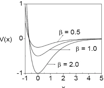
The Morse potential is widely used to provide an approximate potential energy function for diatomic molecules and in polyatomic molecules to describe the potential energy surface along a bond stretching direction [20]. Figure 1 depicts the shape of the potential for a few values of β.
Figure 1. Morse potential curve for three values of βwith α = 1.
the bifurcations of periodic orbits and chaos in damped and driven Morse oscillator both analytically and numerically. Behnia et al. [30] investigated the control of chaos in damped and driven Morse oscillator via slave-master feedback. Gan et al. [31] investigated the torus breakdown and noise induced dynamics in the randomly driven Morse oscillator. de Lima [32] studied the control of chaotic photodissociation in the classical driven Morse oscillator by means of bichromatic pulses. Recently, Abirami et al. [33] have investigated the occurrence of vibrational resonance in both classical and quantum mechanical Morse oscillators driven by a biharmonic force.
This paper is organized as follows. In section 2 we analyze the occurrence of VR in classical Morse oscillator driven by NBFM signal and with WBFM signal in section 3. We characterized VR and dynamics of the system using response amplitude Q and bifurcation diagram. In the final section we summarized and discuss results of this work.
2. VIBRATIONAL RESONANCE WITH NBFM SIGNAL
That is single resonance occurs in the interval 0 < g < 1120.9747. For g > 1120.9747, multiple resonances occur. For β = 0.5, Qdecreases continuously with g. This is shown in
Fig. (2c). Figure 3 shows the variation of the response amplitude Qwith g for fixed values of
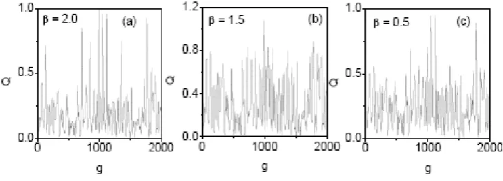
β namely β = 2.0, 1.5, 0.5 and f = 0.5 (chaotic region). VR phenomenon can be observed even in chaotic region. In Fig. 3, when the value of β decreases, the number of resonances was
found to decrease with increase in g. For β = 2.0 and 1.5, multiple resonances occurred in the vast region [Fig. 3(a) and 3(b)] but for β = 0.5, multiple resonances occurred only in the small region [Fig. 3(c)]. In Fig. 3(c) showed that when g > 150.2947, Qdecreases continuously with g.
Figure 2. Response amplitude Q versus g for three values of β = 2.0, 1.5, 0.5. The other parameters values are f = 0.1 (periodic region), d= 0.5, α = 1.0, ω = 1.0, Ω = 10 ω.
Figure 3. Response amplitude Q versus gfor three values of β = 2.0, 1.5, 0.5. The other parameters values are f= 0.5 (chaotic region), d = 0.5, α = 1.0, ω = 1.0, Ω = 10 ω.
Figure 4 presents the dependence of the response amplitude Qon f for three different values of β namely β = 2.0, 1.5, 0.5 with g = 100(periodic region). The other parameters
Figure 4. Response amplitude Q versus f for three values of β = 2.0, 1.5, 0.5. The other parameters values are g= 100 (periodic region), d = 0.5, α = 1.0, ω = 1.0, Ω = 10 ω.
Figure 5 shows the variation of the response amplitude Q with f for three values of β and g = 500 (chaotic region). In Fig. 5(a) for β = 2.0, three resonances were take place for 0 <f< 0.425. Multiple resonance takes place for 0.425 <f< 1.0, after that no resonance takes place when f is further varied. For β = 1.5, single resonance takes place for 0 <f< 0.25, after that multiple resonances take place for 0.25 <f< 1.0. No resonance takes place for 1.0 <f< 2.0 [Fig. 5(b)]. For β = 0.5, Q decreases with f and no resonance takes place. This is clearly shown in Fig. 5(c).
Figure 5. Response amplitude Q versus f for three values of β = 2.0, 1.5, 0.5. The other parameters values are g= 500 (chaotic region), d = 0.5, α = 1.0, ω = 1.0, Ω = 10 ω.
The dependence of Q on the frequencies ω and Ω of the NBFM signal is shown in Fig. 6(a). Q versus Ω is plotted in Fig. 6(a) for three values of β namely β = 2.0, 1.5, 0.5 with f = 0.1 and g = 100 (periodic region). Double resonances take place for 0 < Ω < 2.0 and no resonance takes place for 2.0 <f< 10. Qmaxwas almost the same for β = 2.0, 1.5, 0.5. The
Figure 6. Response amplitude Qversus Ω for three values of β. Solid curve for β = 2.0,
dashed curve for β = 1.5 and dotted curve for β = 0.5. (a) f = 0.1, g = 100 (periodic region)
(b) f = 0.5, g = 500 (chaotic region). The other parameters values are d = 0.5, α = 1.0, ω = 1.0.
Figure 7. Response amplitude Qversus ω for threevalues of β. Solid curve for β = 2.0, dashed curve for β = 1.5 and dotted curve for β = 0.5. (a) f = 0.1, g = 100 (periodic region) (b) f = 0.5, g = 500 (chaotic region). The other parameters values are d = 0.5, α = 1.0, Ω = 10.
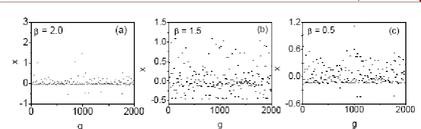
Next we examined the occurrence of variety of bifurcations of periodic orbits leading to chaotic motion and bifurcation of chaotic attractor using bifurcation diagram in system (1) with NBFM signal. For certain cases of the parametric choices considered in our study, periodic and chaotic motions, bifurcations of them were found when the control parameters f and g were varied. An example is presented in Fig. 8 and Fig. 9. In Fig. 8(a) for β = 2.0 and f = 0.1, a period-T solution is found for 0 <f< 1000. When g was varied further period-doubling phenomenon leading to chaotic motion, band merging, intermittency, sudden widening, period-T orbit occur, which are clearly seen in Fig. 8(a). Chaotic orbit disappears at g = 1250 and the long time motion settles to period-T orbit. The bifurcation patterns for β = 1.5 and f = 0.1 is shown in Fig. 8(b). Period-T orbit occurs for 0 <g< 1150 and period - doubling bifurcation takes place for 1250 <g< 1500, which is clearly seen in Fig. 8(b). Only period - T orbit takes place for β = 0.5 [Fig. 8(c)]. For g = 500 (chaotic region) the bifurcation pattern of the system (1) with NBFM signal is shown in Fig. 9. For β = 2.0 and 1.5, period - doubling, chaotic motion and reverse period-doubling bifurcation occurred [Fig. 9(a) and
Figure 8. Bifurcation structures for the system (Eq.1) driven by NBFM signal in (g, x) plane
for three values of β. The other parameters values are d = 0.5, α = 1.0, ω = 1.0, Ω = 10ω and f = 0.1.
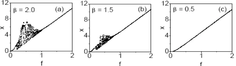
Figure 9. Bifurcation structures for the system (Eq.1) driven by NBFM signal in (f, x) plane for three values of β. The other parameters values are d = 0.5, α = 1.0, ω = 1.0, Ω = 10ω and
g = 500.
3. VIBRATIONAL RESONANCE WITH WBFM SIGNAL.
In this section we show that vibrational resonance can be realized in the Morse oscillator when the external force is a WBFM signal (Eq.2). The variation of Qwith f for three values of β namely β = 2.0, 1.5, 0.5 were shown in fig. 10. In Fig.10 (a), for β = 2.0, 1.5 and g = 100 (periodic region), single resonance takes place for 0 <f< 7.5 with Qmax= 0.14 and 0 <f< 6.5
Figure 10. Response amplitude Q versus f for three values of β = 2.0, 1.5, 0.5. The other parameters values are g= 100 (periodic region), d = 0.5, α = 1.0, ω = 1.0, Ω = 10 ω.
Figure 11 showed the plot of Qagainst g for three values of β namely β = 2.0, 1.5, 0.5 with f = 1.0 (periodic region) and f = 10.0 (chaotic region). The resonance pattern for f = 1.0 is shown in Fig. 11(a) and for f = 10.0 is shown in Fig. 11(b). Next we study the dependence of the response amplitude Q on Ω and ω in system (2) with WBFM signal. Fig 12 shows the plot of Q against Ω for three values of β namely β = 2.0, 1.5, 0.5 with the chosen two values of f and g in the periodic and chaotic regions. Figure 12(a) shows the resonance patterns in the periodic region (f = 1.0, g = 100) and in the chaotic region (f = 10.0, g = 500) shown in
Fig. 12(b). Figures 13(a) and (b) illustrated the variation of numerically calculated Qwith ω for three different values of β namely β = 2.0, 1.5, 0.5 in the periodic region (f = 1.0, g = 100) [Fig. 13(a)] and in the chaotic region (f = 10.0, g = 500) [Fig. 13(b)]. VR phenomenon can be observed in the chaotic region also with considerable enhancement in the weak signal.
Figure 12. Response amplitude Q versus g for three values of β = 2.0, 1.5, 0.5. The other parameters values are f= 1.0, d = 0.5, α = 1.0, ω = 1.0, Ω = 10 ω.
Figure 13. Response amplitude Qversus Ω for three values of β. Solid curve for β = 2.0, dashed curve for β= 1.5 and dotted curve for β = 0.5. (a) f = 0.1, g = 100 (periodic region) (b)
f = 0.5, g = 500 (chaotic region). The other parameters values are d = 0.5, α = 1.0, ω = 1.0.
Then we studied the occurrence of bifurcations of periodic orbits leading to chaotic motion and bifurcations of them in system (2) with WBFM signal. Figure 14 shows the bifurcation diagram of f versus x for three values of β namely β = 2.0, 1.5, 0.5 with g =500 (chaotic region). When f was varied from small values, the system (2) with WBFM signal admits variety of bifurcations such as transcritical, period - doubling, chaos, intermittency, period - bubbling, reverse period - doubling etc, which are clearly seen in Fig. 14. The bifurcation diagram of g versus x for three values of f namely f = 0.1, 1.0, 10.0 with β = 2.0 is shown in Fig. 15. No periodic orbits occur and we observed only chaotic orbits, which are clearly seen in Fig. 15.
Figure 14. Bifurcation structures for the system (Eq. 2) driven by NBFM signal in (f, x) plane for three values of β. The other parameters values are d = 0.5, α = 1.0, ω = 1.0, Ω = 10
Figure 15. Bifurcation structures for the system (Eq.2) driven by NBFM signal in (g, x) plane
for three values of β. The other parameters values are d = 0.5, α = 1.0, ω = 1.0, Ω = 10ω and f = 10.0.
CONCLUSION
In the present work, we report our investigation on the phenomenon of VR in the classical Morse oscillator driven by narrow band and wide band frequency modulated signals. Here we have shown that the amplification of low frequency components of signals by changing the high frequency components of signals through vibrational resonance phenomenon. For the systems (1) and (2) from numerical analysis, multiple resonances found for a range of fixed parameter values when the amplitudes f and g of the NBFM and WBFM signals are varied. Importantly, VR was also observed in the chaotic region in both systems. The dynamics of the system is studied in the presence of NBFM and WBFM signals separately. We have shown the variety of bifurcations in the system driven by both signals. It is also important to investigate the other types of resonances like coherence, ghost, and parametric resonances in the presence of NBFM and WBFM signals. The analysis of VR in nonlinearly damped system and parametrically driven system can provide further insight in the occurrence of VR.
REFERENCES
[1] Landa, P. S. and McClintock, P. V. E., J. Phys. A: Math. Gen., 2000,33, L433 - L438. [2] Gitterman, M., J. Phys . A: Math. Gen., 2001, 34, L355 - L357.
[3] Baltanas, J.P., Lopez, L., Blechman, I.I., Landa, P.S., Zaikin, A., Kurths, J. and Sanjuan, M.A.F., Phys. Rev. E, 2003, 67, 066119 - 1 - 7.
[4] Ullner, E., Zaikin, A., Garcia-Ojalvo, J., Bascones, R., and Kurths, J., Phys. Lett. A, 2003, 312, 348 - 354.
[5] Chizhevsky, V.N., Smeu, E. and Giacomelli, G., Phys. Rev. Lett., 2003, 91, 220602. [6] Jeyakumari, S., Chinnathambi, V., Rajasekar, S. and Sanjuan, M.A.F., Phys. Rev. E.,
2009, 80, 046608.
[7] Jeyakumari, S., Chinnathambi, V.,Rajasekar, S. and Sanjuan, M.A.F., Chaos, 2009, 19, 043128.
[8] Yang, J. H. and Liu, X. B., Phys. Scr., 2010, 82, 025006.
[9] Jeevarathinam, C., Rajasekar, S., and Sanjuan, M. A. F., Phys. Rev. E, 2011, 83, 066205.
[10] Rajasekar, S., Abirami, K., and Sanjuan, M. A. F., Ecol. Complex., 2013, 15, 33-42. [11] Deng, B., Wang, J. and Wei, X., Chaos, 2009,19, 013117.
[12] Deng, B., Wang, J., Wei, X., Tsang, K. M., and Chan, W. L., Chaos, 2010, 20, 013113 [13] Zaikin, A. A., Lopez, L., Baltanas, J. P., Kurths, J. and Sanjuan, M. A. F., Phys. Rev. E,
[14] Rajasekar, S., Used, J., Wagemakers, A., and Sanjuan, M. A. F., Commun. Nonlinear Sci. Numer. Simul.,2012, 17, 3435-3445.
[15] Jeevarekha, A., Santhiah, M. and Philominathan, P., Pramana-J. Phys., 2014, 83(4), 493-504.
[16] Gandhimathi, V.M., Rajasekar, S. and Kurths, J., Phys. Lett. A., 2006,360, 279-286. [17] Ravisankar, L., Ravichandran, V., Chinnathambi, V. and Rajasekar, S., IJSER, 2013,
4(8), 1955-1962.
[18] Ravisankar, L., Ravichandran, V., Chinnathambi, V. and Rajasekar, S., CJP, 2014, 52(3), 1026-1043.
[19] Lai, Y. C., Liu, Z., Nachman, A. and Zhu, L., Int. J. Bifurcation Chaos, 2004, 14, 3519-3539.
[20] Morse, P. M., Phys. Rev., 1929,34, 57-64.
[21] Ackerhalt, J. R. and Milonni, P. W., Phys. Rev. A., 1986, 34, 1211. [22] Goggin, M. E. and Milonni, P. W., Phys. Rev. A, 1988, 37, 796-806. [23] Dardi, P. S. and Gray, S. K., J. Chem. Phys., 1982, 77(3), 1345-1353. [24] Beigie, D. and Wiggins, S., Phys. Rev. A, 1992, 45(7), 4803-4827. [25] Memboeuf, A. and Aubry, S., Physica D, 2005, 207, 1-23.
[26] Gray, S. K., Chem. Phys., 1983, 75(1), 67-78.
[27] Lie, G. C. and Yuan, J., J. Chem. Phys., 1986, 84, 5486-5493.
[28] Knop, W. and Lauterborn, W., J. Chem. Phys.,1990, 93(6), 3950-3957. [29] Jing, Z., Deng, J. and Yang, J., Chaos, Solitons Fractals, 2008, 35, 486-505. [30] Behnia, S., Akhshani, A., Panahi, M., and Asadi, R., Acta Phys. Pol. A, 2013, 123(1), 7-12.
[31] Gan, G., Wang, Q. and Perc, M., J. Phys. A: Math. Theor.,2010, 43, 125102 (13pp). [32] de Lima, E. F., PHYSCON 2011, Leon, Spain, Sep. 5 - Sep. 8, 2011.