ANALIZING DENSITY AND ENVIRONMENTAL FACTORS OF THE JAVA SEA PELAGIC FISH USING CATCH, REMOTE SENSING, AND HYDRO ACOUSTIC DATA

(1)

ANALIZING DENSITY AND ENVIRONMENTAL FACTORS OF THE JAVA

SEA PELAGIC FISH USING CATCH, REMOTE SENSING, AND HYDRO ACOUSTIC DATA

Wijopriono

Research Institute for Marine Fisheries, Muara Baru-Jakarta

Received April 4-2007; Received in revised form June 11-2007; Accepted August 9-2007

ABSTRACT

The relationship between the variations in density of pelagic fish in the Java Sea and a suite of variables describing the environment was studied. The indicator of density (local fish abundance) used were catch per unit of effort, obtained from 1,198 catches made by commercial fishing during the 5 year period (1998 until 2002), and number of fish per unit of area from acoustic investigation made in 2002. The set of environmental parameters included: temporal (monsoon), spatial (Longitude), and productivity level and thermal conditions of the environment (plankton, chlorophyll-a, sea surface temperature). Multivariate modelling and geographic information system modelling approaches were adopted to identify relationships between catch per unit of effort and each environmental variable. Using multivariate modelling approach, the environmental variables explained 46.5% of the variation in catch per unit of effort of pelagic fish in the final general linier models. Temporal variable (monsoon) and thermal conditions of the environment (sea surface temperature) accounted for the major parts of the variability in catch per unit of effort.Model results further indicated that pelagic fish prefer water cooler than 28°C. Geographic information system model has demonstrated its capability in delineating spatial patterns of fish densities in relation to environmental variables, especially zooplankton.

KEYWORDS: density, GIS, GLM, pelagic fish, Java Sea

INTRODUCTION

Pelagic fishery in the Java Sea is multispecies and dominated by a community of small pelagic species, which have undergone considerable variations in both their distributions and abundances over time. The fishery stocks supported annual catch of more than a hundred thousand tons in 1985, but several years of poor catches occurred before back to the similar level in 1992 (Potier & Sadhotomo, 1995). They are most abundant in August until September, decreasing in November and drop to the lowest level in February.

A growing body of evidence suggests that the environmental factors play a dominant role in the processes changing the abundances of small pelagic fish around the world. For instance, during the 1972 until 1973 and 1976 until 1977 ENSOs, sardine availability dropped drastically along the coast of Sonora (Nevarez-Martinez et al., 2001). Similar oscillations occurred in anchovy fisheries and pacific sardine stocks (Clark & Marr, 1955; Kondo, 1980; Radovich, 1982; Hayasi, 1983; Kawasaki & Omori, 1988; Lluch-Belda et al., 1989; Nevarez-Martinez et al., 2001). Environmental factors have also been recognized as a determinant of recruitment success, distribution and migration patterns (Harden Jones, 1968; Laevastu & Hayes, 1981; Cury et al., 2000). Understanding the effects of environmental forcing on the different development stages may be crucial to

effective exploitation management of these fish resources which are subject to such large population fluctuations on seasonal and inter annual scales. Environmental conditions, however, also influence fishing operations on shorter temporal scales, by affecting the distribution and local abundance of fish within the fishing grounds. A better understanding of such influences is therefore of considerable financial value to the fishing industry because such knowledge will assist them to reduce the time and fuel expended by the boats in search of fish concentrations. From a resource management point of view, the ensuing greater efficiency of the commercial operations is important as it would, at least in principle, help to make operations more profitable and thus increase the viability of smaller allocation in particular.

(2)

Fishers have empirically known that fishes aggregate in certain regions characterized by traditional indicators of ocean features (temperature and water colour, feeding birds, and floating objects). In fact, several investigation using remote sensing and hydroacoustics information have shown the distribution and availability of fish are related to the ocean variability (Montgomery et al., 1986; Perry & Smith, 1994; Demarcq & Faure, 2000). The ocean variables, including sea surface temperature and chlorophyll-a, then have been used to predict the distribution of fishes and ocean phenomena such as fronts, eddies and coastal upwelling cells have been used as the indicators of high productivity area (Lasker et al., 1981; Laurs et al, 1991). They are both important ocean processes biologically and of which are available with good spatial and temporal resolution from two decades of satellite generated data.

In the case of small pelagic species, the relationship with sea surface temperature is not as clear as for large pelagic fish. Anchovy spawning, for example, is thought to be related to certain temperature ranges (Lasker et al., 1981; Fiedler, 1983; Richardson et al., 1998; Van der Lingen et al., 2001), while in the North Sea greater densities of herring are associated with gradients of sea surface temperature and salinity (Maravelias & Reid, 1995). A similar association of anchovy, sardine and jack mackerel distributions with thermal fronts was demonstrated in northern Chile (Castillo et al., 1996). But there were also a number of studies that have failed to find a relationship between small pelagic fish and sea surface temperature. For example, the spawning distribution of the Californian anchovy was related to temperature in some studies (Fiedler, 1983), but poorly in others (Lasker et al., 1981). In South Africa, Kerstan (1993) could only explain 2 to 10% of the variance in sardine population density from several environmental variables (including sea surface temperature). Although there are no strong and scientifically proven relationships between sea surface temperature and pelagic fish distributions, satellite thermal images are nonetheless quite commonly used by pelagic fishing fleets in an attempt to locate the best fishing locations.

This study aims to gain a better understanding of the environmental preferences of the main pelagic species and to express these preferences as mathematical functions which may be used in conjunction with sea surface temperature and chlorophyll-a images to predict the locations of fish density.

MATERIALS AND METHODS

Data Collection

Data on pelagic fish density are available from two sources, i.e. from scientific hydro acoustic survey and from records of commercial catches. There are biases associated with both sources, with hydro acoustic survey having good spatial but poor temporal coverage, where as commercial catches tend to have good temporal but poorer spatial coverage.

Commercial catch data were collected from Pekalongan, which constitute a main fishing port for pelagic fishing in the north coast of Java. Data on catch weight, fishing time, and locations of every catch by purse seiners in the pelagic fishing fleet were recorded. The investigation was limited to the period 1998 until 2002 for which satellite data were available and for this period 1,198 catch records were available. Because the exact geographical co-ordinates were often not known for fishing ground positions, they were recorded in terms of a grid system, which divides the fishing grounds into 10’ latitude x 10’ longitude squares. Catch records were then grouped based on the season (month).

Data on hydroacoustic were collected from the survey on September until October 2002. Concomitant data on oceanographic variables were also measured during this survey, covering 60 oceanographic stations (Figure 1). The variables included sea surface temperature, chlorophyll-a, and plankton.

Sea surface temperatures derived from AVHRR GAC data with 4 km spatial resolution were provided through the AVHRR pathfinder-5 while SeaWiFS GAC data (5 km resolution) were provided by the SeaWiFS project. Both data are distributed by Goddard Space Flight Center of the National Aeronautics and Space Administration.

(3)

Figure 1. Geographical position of oceanographic stations and hydro acoustic transect lines made in the survey of September until October 2002.

Data Analysis

The commercial catch data, which contained information on the time, location, catch weight, together with sea surface temperature and chlorophyll-a derived from satellite data were used to build mathematical model of functional relationships between fish and environmental variables. For this purpose, general linier model procedures, which are multivariate model building procedures, were employed.

In order to strengthen the estimation, hydro acoustic together with water temperature, chlorophyll-a and plankton which were derived from in situ measurement, was also used to examine spatial relations between fish density distribution and oceanographic variables. Geographical information system technique was employed for this purpose.

General Linear Model

Predictors

The suite of predictors included those related to the time and location of the catches, and environmental variables. The latter group consisted of sea surface temperature and chlorophyll-a, the variables which are known linked to variations in catch size through biologically meaningful processes. Although a plethora of other variables such as oxygen concentration, food abundance, and reproduction activity could also play a role in fish distributions, however, there were no in situ data available on appropriate time and space scales. Parameters used in the general linier model analysis are summarized in Table 1.

Table 1. A summary of the parameters used in the general linier model analysis

0.11; 0.92

Longitude of the catch

Longitude

Northwest; Southeast

-Monsoon of the catch

Longitude of the catch

Longitude

Northwest; Southeast

(4)

To identify relationship between pelagic catch (catch per unit of effort) and the suite of predictors describing the environment, multiple linier regression model was used. The general form of the linier model is given by:

ε

Variable Y = the response X_i = the predictors

α and β = constants

ε = the errors or the departure term

A multiple regression model is a model in which a response variable Y is linked to p (≥1) predictor variables Xp and a random departure term. The model is linier if it is linier in the parameters, and the link between predictor variables and departure term is most commonly an additive one (Krzanowski, 1998). The departure term ε is independent random variable having mean zero and variance σ2_{. The predictor variables in multiple regression} are taken to be fixed and not random variables. By implication, the only random variable is the response variable Y, and the additional assumption of normality is necessary. The stepwise regression is discibed in Appendix 1.

As the distribution of the response skew to the right, we used a log normal distribution, which has also been recommended in other studies (Hilborn & Walters, 1992; Myers at al., 1995). For checking violation of assumptions, we used analysis of residuals graphically (Krzanowski, 1998; Millard & Neerchal, 2001). Removing low contribution variables in general linier model was validated using stepwise procedure and the Akaike information criterion (Akaike, 1973) was used to define the optimal model. Models are compared according to their Akaike information criterion values; a better model has a lower Akaike information criterion.

Geographical Information System Model

Contour maps of pelagic fish distribution and oceanographic variables were built to develop geographic information system model. Contours map of pelagic fish distribution was built based on hydro acoustic data. The first step was to divide the transects into 5 nmi long segments and for each of these an echo integration value

calculated. The geographical position of the segments was set to their mid-point. From these positions and the echo integration values, linier variogram values were calculated using version 8 of surfer programme. Different models were tried to fit these variogram values, and the best fitting model, by means of krigging (Clark, 1987), was used to interpolate echo integration values for the entire study area. The values from the best fitting model were used to draw contour maps over the distribution of pelagic fish. Contour maps of oceanographic variables (water temperature, chlorophyll-a, and plankton) were built in similar way. They were each then superimposed over the map of the fish density distribution and subjected to geographical base map. Visual analysis was done on these developed maps to examine spatial relations between fish density distribution and oceanographic variables.

Results and Discussion

Models of pelagic fish abundance and environment General Linier Model

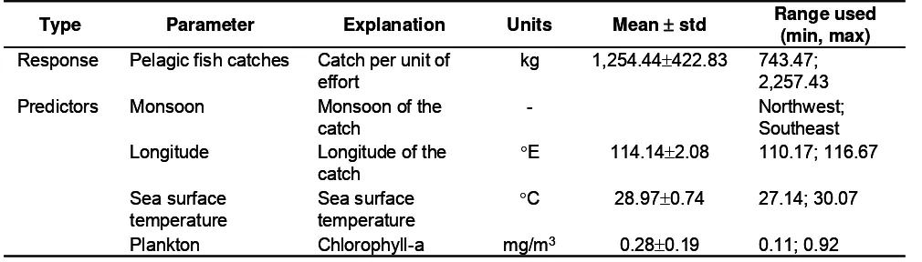
The bivariate general linier model models developed to explore functional relationships between pelagic fish abundance and each environmental variable are shown in Figure 2. We used continuous predictors in the model, however, monsoon, as a categorical predictor, was included in the model in order to account for temporal effect.

Different shapes on the functional relationships between response and each predictor variable were showed. The relationships between response (log catch per unit of effort) and sea surface temperature was linier and negative while with the other predictors it was curve indicating the 2th_{polynomial orders.}

(5)

Figure 2. Bivariate general linier models showing the relationships of response and individual predictors; solid line is the fitted model and dashed lines are 95% confidence intervals.

The optimal model produced from the stepwise analysis involved the single effect of all variables input and also cross effect between chlorophyll-a and longitude. The model equation mathematically is given by:

Log(CPUE)=3.41+á-0.05*SST+10.5*Chla+0.01* Longitude-1.3*Chla2_-0.08*

(Longitude: Chla) ………..……….. (2

where:

SST = sea surface temperature Chla = chlorophyll-a

a = parameter value for monsoon categorical variable where the value is 0.05 for southeast monsoon and zero for northwest monsoon

It is more relevant to consider the relative contributions of the predictors, as provided by the general linier models and summarized in Table 2, to judge the meaning of a factor in the model. General linier model explain 46.5% of the total variance of catch per unit of effort. These were obtained after introduction of interaction (cross effect) between chlorophyll-a and longitude, which gave significant contribution to the model. Without interaction the general linier model explain 39.6% of the variance.

Table 2. Percentage of variance explained by the general linier model parameters (obtained from the general linier model variance table)

46.5 Total

13.3 Monsoon

6.

1.4 Longitude

5.

6.9 Chla: longitude

4.

10.5 Chlorophyl-a

3.

_a Sea surface temperature: longitude

2.

14.4 Sea surface temperature

1.

% of variance explained Variable

No.

46.5 Total

13.3 Monsoon

6.

1.4 Longitude

5.

6.9 Chla: longitude

4.

10.5 Chlorophyl-a

3.

_a Sea surface temperature: longitude

2.

14.4 Sea surface temperature

1.

% of variance explained Variable

No.

(6)

Sea surface temperature and chlorophyll-a (oceanographic variables) explain 14.4 and 10.5% of the total variance of catch per unit of effort, while monsoon (temporal variable) and longitude (spatial variable) variables explain 13.3 and 1.4% of the total variance of catch per unit of effort, respectively. Of the total variance explained by the general linier model predictors, oceanographic variables contribute 54%, confirming the relative importance of these variables in predicting pelagic fish catch. The greatest contribution was made by sea surface temperature (31%).

Geographic Information System Model

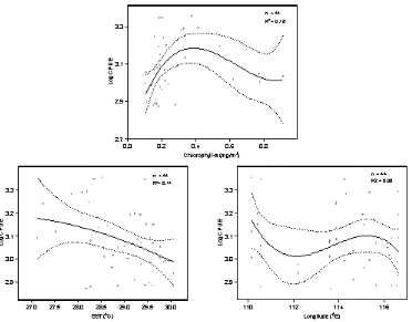
Results of geographic information system model are presented in the form of spatial maps delineating spatial patterns of density distribution of pelagic fishes in relation with their environment. Figure 3 shows spatial relations of the density distribution of pelagic fishes against sea surface temperature and zooplankton during pre northwest monsoon.

It can be seen from the figure that in northwestern of the study area, high densities of the fish concentrated in the area with relatively low temperatures (27.9°C) and high density of zooplankton (20x103_ind.m-3_{). While in} westernmost of the study area, the high densities occurred in higher and wider range of temperatures, i.e. between 28.1°C and 29°C, with relatively lower concentrations of zooplankton (10x103_ind.m-3_{). However,} fish densities in westernmost of the study area were lower than those in the northern one and they decreased to the south.

Spatial relations between density distribution of the fish and both zooplankton and temperature seem to be pronounced. Density of the fish tends to be high in the areas of high concentrations of zooplankton and relatively low temperature and inversely, it is low in the areas with the low concentrations of zooplankton and relatively high temperature.

(7)

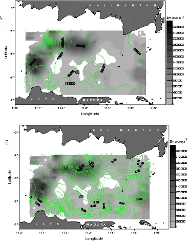
Figure 4 shows spatial relations of the density distribution of pelagic fishes against phytoplankton and chlorophyll-a. High densities of the fish exhibited to distribute within the wide ranges of phytoplankton and chlorophyll-a concentrations, hence, specific relation patterns were apparently less pronounced. However,

taking into account the temperature distributions (Figure 4a), the relations were more pronounced; highest density of fish occurred in the areas with relatively high concentrations of phytoplankton and chlorophyll-a with low temperatures.

(8)

Density of Pelagic Fish

Temporal effect (monsoon) accounts for 13.3% of the total variance (29% of the variance explained by the general linier model), which indicates a strong seasonal effect, and it means that the variance of catch per unit of

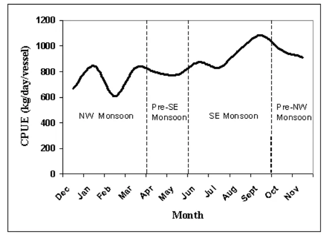
effort is not a fix pattern but change seasonally. During northwest monsoon (December to March), the catch per unit of effort shows fluctuating at relatively low values and it increases during southeast monsoon (June to September), which reaching a peak at the end of the monsoon (Figure 5).

Figure 5. Mean seasonal variability of pelagic fish catches in the Java Sea.

Based on reproductive biology investigation, spawning season of pelagic fishes in the Java Sea varies between species. For the dominant pelagic species, Decapterus spp., the spawning season occurred from May to December (Atmaja et al., 1995). Length at first capture (l_c) is 14.8 to 16.3 cm, which corresponds to about 1 year old (Suwarso,B. Sadhotomo, & S. B. Atmadja 1995; Widodo, 1995). This indicates that the fish biomass would be abundant during the southeast monsoon. The catch per unit of effort and fish biomass seem to have a similar trend and therefore leads us to surmise that the influence of the season parameter is at least partly derived from a relationship between catch per unit of effort and population size as was previously reported for other pelagic fisheries (Freon, 1991; Wada & Matsumiya, 1990). The spatial predictor, longitude, essentially indicates the variation of catch per unit of effort from west fishing ground to the east. Positive trend is showed from the waters around Masalembo to Kangean, Matasiri but continuing to the

east the trend is inversely negative. High catch per unit of effort is also showed in the westernmost fishing ground (Figure 2).

(9)

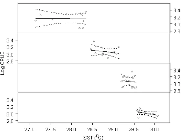
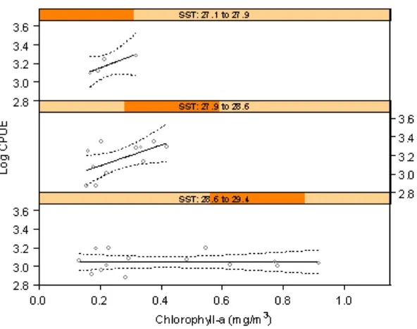
Relationship between fish catches and chlorophyll-a in the general linier model model (equation 1) show a positive relation in 1st_{order but negative for 2}nd_{order. The} discrepancy can be explained through trellis graph in Figure 7. Taking into account the sea surface temperature as a condition factor, effect of chlorophyll-a on the catches seems to be more pronounced.

As can be seen from the figure, a positive trend was exhibited with increasing chlorophyll-a in temperature range of less than 28.5°C. The curve was flat in the lowest level of the catches in temperature of more than 28.5°C, indicating the chlorophyll-a having no effect on the fish catches. The interaction between chlorophyll-a and longitude was included in the model, accounting for spatial variability; the effect is only moderate, indicating that the chlorophyll-a relationship is spatially fairly stable.

Spatial map of geographic information system model indicates a positive relation between fish density and zooplankton abundance. In other words, pelagic fishes tend to inhabit the area with high zooplankton abundance.

Figure 6. Relationship between pelagic fish catches and sea surface temperature in the different ranges of sea surface temperature.

This is not surprisingly since zooplankton is the main food item most of pelagic fishes (Mann & Lazier, 1991; Kornilovs et al., 2001) specifically for Decapterus spp., Rastrelliger spp., and Selar crumenophthalmus (Widodo, 1995). Moreover, it agrees with the results of investigation done by Wiadnyana (1997) which found that highest abundance of pelagic fishes in Kao Bay, Moluccas, occurred at the time after the peak abundance of zooplankton.

(10)

Figure 7. Relationship between pelagic fish catches and chlorophyll-a in different ranges of sea surface temperature.

It was recognized that catch per unit of effort is only an approximation of school size and that factors such as characteristic of fishing gear, fishing tactics, and skill of the skippers, which difficult to account for, may affect catch size. Design of fishing gears is different among the vessels depending on the preference and practices of each skipper. It is also different between the vessels operated in relatively shallow and deeper waters. The pelagic fleets use fish aggregating device, i.e. rumpon and light for attracting and gathering fish schools in their fishing tactics. The fleets use different power of light, ranging from 12 to 36 halogen floodlights of 200 to 600 watts. The influence of light on the fish catches in pelagic fishing has been confirmed to be positive (Potier & Sadhotomo, 1995). There are also many other factors that affect this approximation but for which we cannot compensate in this models, such as recruitment pattern or fish stocks, dissolve oxygen, and moon phase or fishing time.

Conclusions and Recommendations

Temporal effect (monsoon) accounts for 13.3% of the total variance or 29% of the variance explained by the general linier model, which indicates a strong seasonal effect and it means that the variance of catch per unit of effort is not a fix pattern but change seasonally. General linier model gives also evidence that the pelagic fish species of the Java Sea have a temperature preference, i.e. cooler than about 28°C, and up to this temperature

limit they have a positive trend of relationships with chlorophyll-a concentration. A part from this, geographic information system model has demonstrated its capability in delineating spatial patterns of fish densities in relation to environmental variables, especially zooplankton, which does not covered in the general linier model.

With the advance of satellite remote sensing technology, sea surface temperature and chlorophyll-a derived data have been provided in a regular basis. In the other side, prediction of potential fishing zones by using these data has now been of a great interest of many fisheries stakeholders. Owing to the results of this study, sea surface temperature and chlorophyll-a derived data should be used in complement when predicting potential fishing zones of pelagic fishes in the Java Sea, as this would increase the predicting precision.

(11)

precisely the distributions of pelagic fish species and relations to their environment and that is crucial for sustainable fisheries management.

ACKNOWLEDGEMENTS

This paper was part of the result of bioecology and assessment of fishery resources in the Java Sea research, funded under state budget of Research Institute for Marine Fisheries 2002 and 2005 scheme.

REFERENCES

Akaike, H. 1973. Information theory and an extension of the maximum likelihood principle. In Second International Symposium on Information Theory, ed. B. N. Petrov & F. Csaki. pp. 267-281. Budapest: Akademia Kiado.

Atmaja, S. B., B. Sadhotomo, & Suwarso. 1995. Reproduction of the main small pelagic species. In BIODINEX. ed. M. Potier & S. Nurhakim. pp 69-84. Jakarta. AARD-ORSTOM-EU.

Castillo, J., M. A. Barbieri, & A. Gonzales. 1996. Relationship between sea surface temperature, salinity, and pelagic fish distribution off northern Chile. ICES Journal of Marine Science. 53: 139-146. Clark, I. 1987. Practical geostatistics. New York: Elsevier

Applied Science.

Clark, I. N. & J. C. Marr. 1955. Population dynamics of the Pacific sardine. CalCOFI Progress Report. 4-52. Cury, P., A. Bakun, R. J. M. Crawford, A. Jarre, R. A. Quinones, L. J. Shannon, & H. M. Verheye. 2000. Small pelagic in upwelling systems: Patterns of interaction and structural changes in wasp waist ecosystems. ICES Journal of Marine Science. 57: 603-618.

Demarcq, H. & V. Faure. 2000. Coastal upwelling and associated retention indices derived from satellite sea surface temperature. Application to Octopus vulgaris recruitment. Oceanologica Acta. 23: 391-408. Fiedler, P.C. 1983. Satellite remote sensing of the habitat

of spawning anchovy in the southern California Bight. CalCOFI Report. 24: 202-209.

Freon, P. 1991. Seasonal and interannual variations of mean catch per set in Senegalese sardine fisheries: Fish behaviour of fishing strategy? In T. Kawasaki, S.

Tanaka, Y. Toba, & A. Tanigushi (Eds), Long-term variability of pelagic fish populations and their environment. pp. 135-145. Oxford. Pergamon Press.

Harden Jones, F. R. 1968. Fish migration. London. Arnold Ltd.

Hayasi, S. 1983. Some explanation for changes in abundance of major neritic pelagic stocks in the northwestern Pacific Ocean. FAO Fisheries Report. 291: 37-55.

Hilborn, R. & C. J. Walters. 1992. Quantitative fisheries stock assessment. Change, dynamics, and uncertainty. New York. Chapman and Hall.

Kawasaki, T. & M. Omori. 1988. Fluctuations in the three major sardine stocks in the Pacific and the global trend in temperature. In Long term changes in marine fish populations, ed. T. Wyatt & M. G. Larrencta, pp 37-53.Vigo. Espana. Instituto de Investigaciones Marinas de Vigo.

Kerstan, S. 1993. Relationships between pilchard distribution and environmental factors. Paper presented at the 8th_{South African Marine Science}

Symposium, Langebaan, South Africa. 17-22 October 1993.

Kondo, K. 1980. The recovery of Japanese sardine the biological basis of stock-size fluctuations. Rapports et Proces Verbaux des Reunions du Conseil Internationale pour l’Exploration de la Mer 177: 332-354.

Kornilovs, G., L. Sidrevics, & J. W. Dippner. 2001. Fish and zooplankton interaction in the Central Baltic Sea. ICES Journal of Marine Science. 58: 579-588. Krzanowski, W. J. 1998. An introduction to statistical

modelling. London. Arnold.

Laevastu, T. & M. L. Hayes. 1981. Fisheries oceanography and ecology. Farnham: Fishing News (Books).

Lasker, R., J. Palaez, & R. M. Laurs. 1981. The use of satellite imagery for describing ocean processes in relation to spawning of the northern anchovy (Engraulis mordax). Remote Sensing of the Environment. 11:439-453.

(12)

Subarctic Frontal Zone. ed.J. A. Wetherall. pp 69– 87. NOAATechnical Report. NMFS 105.

Lluch-Belda, D., J. M. Crawford, T. Kawasaki, A. D. MacCall, R. H. Parrish, R. A. Schwartzlose, & P. E. Smith. 1989. Worldwide fluctuations of sardine and anchovy stocks: The regime problem. South African Journal of Marine Science. 8: 195-205.

Mann, K. H. & J. R. N. Lazier. 1991. Dynamics of marine ecosystems: Biological physical interactions in the sea. Boston: Blackwell Scientific Publications.

Maravelias, C. D. & D. G. Reid. 1995. Relationship between herring (Clupea harengus, L.) distribution and sea surface temperature in the northern North Sea. Scientia Marina. 59: 427-438.

Millard, S. P. & N. K. Neerchal. 2001. Environmental statistics with S-Plus. New York. CRC Press. Montgomery, D. R., R. E. Wittenberg, & R. W. Austin.

1986. The applications of satellite derived ocean color products to commercial fishing operations. Marine Technological Society of Japan. 20(2): 72-86.

Myers, R. A., J. Bridson, & N. J. Barrowman. 1995. Summary of world wide spawner and recruitment data. Canadian Special Publication of Fisheries and Aquatic Science.327: 2024.

Nevarez-Martinez, M. O., D. Lluch-Belda, M. A. Cisneros-Mata, J. P. Santos-Molina, M. D. A. Martinez-Zavala, & S. E. Lluch-Cota. 2001. Distribution and abundance of the Pacific sardine (Sardinops sagax) in the Gulf of California and their relation with the environment. Progress in Oceanography. 49: 565-580.

Perry, R. I. & S. J. Smith. 1994. Identifying habitat associations of marine fishes using survey data: An application to the Northwest Atlantic. Canadian Journal of Fisheries and Aquatic Science. 51: 589-602.

Potier, M. & B. Sadhotomo. 1995. Exploitation of the large and medium seiners fisheries. InBIODINEX. ed. M. Potier & S. Nurhakim. pp 195-214. Jakarta. AARD-ORSTOM-EU.

Radovich, J. 1982. The collapse of the California sardine fisheries: What have we learned? CalCOFI Report. 23: 56-78.

Richardson, A. J., B. A. Mitchell-Innes, J. L. Fowler, S. F. Bloomer, J. G. Field, H. M. Verheye, L. Hutchings, & S. J. Painting. 1998. The effect of sea temperature and food availability on the spawning success of the Cape anchovy Engraulis capensis in the southern Benguela. South African Journal of Marine Science. 19: 275-290.

Suwarso, B. Sadhotomo, & S. B. Atmaja. 1995. Growth parameters of the main small pelagic species. In BIODINEX, ed. M. Potier & S. Nurhakim. pp 85-96. Jakarta. AARD-ORSTOM-EU.

Van der Lingen, C. D., L. Hutchings, D. Merkle, J. J. Van der Westhuizen, & J. Nelson. 2001. Comparative spawning habitats of anchovy (Engraulis capensis) and sardine (Sardinops sagax) in the southern Benguela upwelling ecosystem. InSpatial processes and management of marine populations, ed. G. H. Kruse, N. Bez, T. Booth, M. Dorn, S. Hills, R. N. Lipcius, D. Pelletier, C. Roy, S. J. Smith, & D. Witherell. pp. 185-209. Fairbanks. University of Alaska Sea Grant. AK-SG-01-02.

Wada, T. & T. Matsumiya. 1990. Abundance index in purse seine fishery with searching time. Nippon Suisan Gakkaishi. 56: 725-725.

Wiadnyana, N. N. 1997. Variation of zooplankton Abundance in Kao, Halmahera (North Moluccas). Oseanologi dan Limnologi di Indonesia. 30: 53-62. Widodo, J. 1995. Population dynamics of ikan layang,

(13)

Appendix 1.

Statistical Analysis for General Linier Model

***Stepwise Regression***

***Stepwise Model Comparisons***

Start: AIC=0.7867

LCATCH~Monsoon+SST+CHLA+Long+SST: CHLA+Long: CHLA+CHLA^2+CHLA^3+Monsoon: SST: CHLA+Monsoon: SST+Monsoon: CHLA+SST^2+CHLA^2+SST^3+Long: SST+Long: SST: CHLA

Single term deletions Model:

LCATCH~Monsoon+SST+CHLA+Long+SST: CHLA+Long: CHLA+CHLA^2+CHLA^3+Monsoon: SST: CHLA+Monsoon: SST+Monsoon: CHLA+SST^2+CHLA^2+SST^3+Long: SST+Long: SST: CHLA

scale: 0.01311187

Df Sum of Sq RSS Cp <none> 0.3671324 0.7867122 I(CHLA^2) 1 0.00261927 0.3697516 0.7631077 I(CHLA^3) 1 0.00023179 0.3673641 0.7607202 I(SST^2) 1 0.01781276 0.3849451 0.7783012 I(SST^3) 1 0.01743805 0.3845704 0.7779265 Monsoon:SST:CHLA 1 0.00003950 0.3671719 0.7605280 Long:SST:CHLA 1 0.00225057 0.3693829 0.7627390 Step: AIC=0.7605

LCATCH~Monsoon+SST+CHLA+Lat2+I(CHLA^2)+I(CHLA^3)+I(SST^2)+I(SST^3)+SST: CHLA+Long: CHLA+Monsoon: SST+Monsoon: CHLA+Long: SST+Long: SST: CHLA

LCATCH~Monsoon+SST+CHLA+Long+I(CHLA^2)+I(CHLA^3)+I(SST^2)+I(SST^3)+SST: CHLA+Long: CHLA+Monsoon: SST+Monsoon: CHLA+Long: SST+Long: SST: CHLA

scale: 0.01311187

Df Sum of Sq RSS Cp <none> 0.3671719 0.7605280 I(CHLA^2) 1 0.00292019 0.3700920 0.7372244 I(CHLA^3) 1 0.00028028 0.3674521 0.7345845 I(SST^2) 1 0.01855494 0.3857268 0.7528591 I(SST^3) 1 0.01815850 0.3853304 0.7524627 Monsoon:SST 1 0.01461455 0.3817864 0.7489188 Monsoon:CHLA 1 0.01215100 0.3793229 0.7464552 Long:SST:CHLA 1 0.00228704 0.3694589 0.7365912 Single term additions

Model:

LCATCH~Monsoon+SST+CHLA+Long+I(CHLA^2)+I(CHLA^3)+I(SST^2)+I(SST^3)+SST: CHLA+Long: CHLA+Monsoon: SST+Monsoon: CHLA+Long: SST+Long: SST: CHLA

scale: 0.01311187

Df Sum of Sq RSS Cp <none> 0.3671719 0.7605280 Monsoon:SST:CHLA 1 0.00003950178 0.3671324 0.7867122 Step: AIC=0.7346

LCATCH~Monsoon+SST+CHLA+Long+I(CHLA^2)+I(SST^2)+I(SST^3)+SST: CHLA+Long: CHLA+Monsoon: SST+Monsoon: CHLA+Long: SST+Long: SST: CHLA

(14)

scale: 0.01311187

Df Sum of Sq RSS Cp <none> 0.3674521 0.7345845 I(CHLA^2) 1 0.09549925 0.4629514 0.8038600 I(SST^2) 1 0.01829150 0.3857436 0.7266522 I(SST^3) 1 0.01789695 0.3853491 0.7262577 Monsoon:SST 1 0.01453933 0.3819915 0.7229001 Monsoon:CHLA 1 0.01265682 0.3801090 0.7210176 Long:SST:CHLA 1 0.00280216 0.3702543 0.7111629 Single term additions

Model:

LCATCH~Monsoon+SST+CHLA+Long+I(CHLA^2)+I(SST^2)+I(SST^3)+SST:CHLA+Long: CHLA+Monsoon: SST+Monsoon: CHLA+Long: SST+Long: SST: CHLA

scale: 0.01311187

Df Sum of Sq RSS Cp <none> 0.3674521 0.7345845 I(CHLA^3) 1 0.0002802753 0.3671719 0.7605280 Monsoon:SST:CHLA 1 0.0000879902 0.3673641 0.7607202 Step: AIC= 0.7112

LCATCH~Monsoon+SST+CHLA+Long+I(CHLA^2)+I(SST^2)+I(SST^3)+SST: CHLA+Long: CHLA+Monsoon: SST+Monsoon: CHLA+Long: SST

scale: 0.01311187

Df Sum of Sq RSS Cp <none> 0.3702543 0.7111629 I(CHLA^2) 1 0.09516561 0.4654199 0.7801048 I(SST^2) 1 0.01568954 0.3859438 0.7006287 I(SST^3) 1 0.01531419 0.3855685 0.7002534 SST:CHLA 1 0.01100828 0.3812626 0.6959474 Long:CHLA 1 0.05810182 0.4283561 0.7430410 Monsoon:SST 1 0.01298487 0.3832392 0.6979240 Monsoon:CHLA 1 0.00985548 0.3801098 0.6947946 Long:SST 1 0.01266550 0.3829198 0.6976047 Single term additions

Model:

scale: 0.01311187

Df Sum of Sq RSS Cp <none> 0.3702543 0.7111629 I(CHLA^3) 1 0.000795394 0.3694589 0.7365912 Monsoon:SST:CHLA 1 0.000028000 0.3702263 0.7373586 Long:SST:CHLA 1 0.002802157 0.3674521 0.7345845 Step: AIC=0.6948

LCATCH~Monsoon+SST+CHLA+Long+I(CHLA^2)+I(SST^2)+I(SST^3)+SST: CHLA+Long: CHLA+Monsoon: SST+Long: SST

scale: 0.01311187

(15)

SST:CHLA 1 0.01034698 0.3904567 0.6789179 Long:CHLA 1 0.04837737 0.4284871 0.7169483 Monsoon:SST 1 0.01046877 0.3905785 0.6790397 Long:SST 1 0.01320835 0.3933181 0.6817793 Single term additions

Model:

scale: 0.01311187

Df Sum of Sq RSS Cp <none> 0.3801098 0.6947946 I(CHLA^3) 1 0.000744082 0.3793657 0.7202743 Monsoon:CHLA 1 0.009855483 0.3702543 0.7111629 Long:SST:CHLA 1 0.000000822 0.3801090 0.7210176 Step: AIC=0.6789

LCATCH~Monsoon+SST+CHLA+Long+I(CHLA^2)+I(SST^2)+I(SST^3)+Long: CHLA+Monsoon: SST+Long: SST

scale: 0.01311187

Df Sum of Sq RSS Cp <none> 0.3904567 0.6789179 I(CHLA^2) 1 0.1249959 0.5154527 0.7776901 I(SST^2) 1 0.0118924 0.4023492 0.6645866 I(SST^3) 1 0.0115623 0.4020190 0.6642564 Long:CHLA 1 0.0388470 0.4293037 0.6915411 Monsoon:SST 1 0.0143240 0.4047807 0.6670181 Long:SST 1 0.0126542 0.4031109 0.6653483 Single term additions

Model:

scale: 0.01311187

Df Sum of Sq RSS Cp <none> 0.3904567 0.6789179 I(CHLA^3) 1 0.00002509 0.3904317 0.7051165 SST:CHLA 1 0.01034698 0.3801098 0.6947946 Monsoon:CHLA 1 0.00919418 0.3812626 0.6959474 Step: AIC=0.6643

LCATCH~Monsoon+SST+CHLA+Long+I(CHLA^2)+I(SST^2)+Long: CHLA+ Monsoon: SST+Long: SST

LCATCH~Monsoon+SST+CHLA+Long+I(CHLA^2)+I(SST^2)+Long: CHLA+Monsoon: SST+Long: SST

scale: 0.01311187

Df Sum of Sq RSS Cp <none> 0.4020190 0.6642564 I(CHLA^2) 1 0.1271493 0.5291683 0.7651820 I(SST^2) 1 0.0303444 0.4323634 0.6683770 Long:CHLA 1 0.0441460 0.4461650 0.6821787 Monsoon:SST 1 0.0046751 0.4066941 0.6427078 Long:SST 1 0.0066130 0.4086320 0.6446457 Single term additions

Model:

LCATCH~Monsoon+SST+CHLA+Long+I(CHLA^2)+I(SST^2)+Long: CHLA+Monsoon: SST+Long: SST

scale: 0.01311187

(16)

<none> 0.4020190 0.6642564 I(CHLA^3) 1 0.00003896 0.4019800 0.6904412 I(SST^3) 1 0.01156225 0.3904567 0.6789179 SST:CHLA 1 0.00462565 0.3973933 0.6858545 Monsoon:CHLA 1 0.01098642 0.3910326 0.6794937 Step: AIC=0.6427

LCATCH~Monsoon+SST+CHLA+Long+I(CHLA^2)+I(SST^2)+Long: CHLA+Long: SST

scale: 0.01311187

Df Sum of Sq RSS Cp <none> 0.4066941 0.6427078 Monsoon 1 0.1327216 0.5394157 0.7492056 I(CHLA^2) 1 0.1477638 0.5544579 0.7642479 I(SST^2) 1 0.0266995 0.4333936 0.6431835 Long:CHLA 1 0.0463021 0.4529962 0.6627862 Long:SST 1 0.0049043 0.4115984 0.6213883 Single term additions

Model:

scale: 0.01311187

Df Sum of Sq RSS Cp <none> 0.4066941 0.6427078 I(CHLA^3) 1 0.000066262 0.4066278 0.6688652 I(SST^3) 1 0.001913361 0.4047807 0.6670181 SST:CHLA 1 0.007860401 0.3988337 0.6610711 Monsoon:SST 1 0.004675096 0.4020190 0.6642564 Monsoon:CHLA 1 0.007491145 0.3992030 0.6614403 Step: AIC=0.6214

LCATCH~Monsoon+SST+CHLA+Long+I(CHLA^2)+I(SST^2)+Long: CHLA

scale: 0.01311187

Df Sum of Sq RSS Cp <none> 0.4115984 0.6213883 Monsoon 1 0.1280535 0.5396518 0.7232180 SST 1 0.0235958 0.4351941 0.6187603 I(CHLA^2) 1 0.1462609 0.5578593 0.7414254 I(SST^2) 1 0.0227872 0.4343856 0.6179518 Long:CHLA 1 0.0461024 0.4577008 0.6412669 Single term additions

Model:

scale: 0.01311187

Df Sum of Sq RSS Cp <none> 0.4115984 0.6213883 I(CHLA^3) 1 0.000298074 0.4113003 0.6473140 I(SST^3) 1 0.000974250 0.4106241 0.6466378 SST:CHLA 1 0.007853130 0.4037452 0.6397589 Monsoon:SST 1 0.002966379 0.4086320 0.6446457 Monsoon:CHLA 1 0.007941774 0.4036566 0.6396703 Long:SST 1 0.004904278 0.4066941 0.6427078 Step: AIC= 0.618

LCATCH~Monsoon+SST+CHLA+Long+I(CHLA^2)+Long: CHLA

(17)

scale: 0.01311187

Df Sum of Sq RSS Cp <none> 0.4343856 0.6179518 Monsoon 1 0.1092403 0.5436259 0.7009683 SST 1 0.0438123 0.4781979 0.6355404 I(CHLA^2) 1 0.1246965 0.5590821 0.7164246 Long:CHLA 1 0.0556814 0.4900670 0.6474094 Single term additions

Model:

LCATCH~Monsoon+SST+CHLA+Long+I(CHLA^2)+Long: CHLA

scale: 0.01311187

Df Sum of Sq RSS Cp <none> 0.4343856 0.6179518 I(CHLA^3) 1 0.00130011 0.4330855 0.6428754 I(SST^2) 1 0.02278724 0.4115984 0.6213883 I(SST^3) 1 0.02268432 0.4117013 0.6214912 SST:CHLA 1 0.01033499 0.4240506 0.6338405 Monsoon:SST 1 0.00076376 0.4336219 0.6434118 Monsoon:CHLA 1 0.00467183 0.4297138 0.6395037 Long:SST 1 0.00099206 0.4333936 0.6431835

***Linear Model***

Call: lm(formula = LCATCH~Monsoon+SST+CHLA+Long+I(CHLA^2)+Long: CHLA Data = CatchSSTChlor, na.action = na.exclude)

Residuals:

Min 1Q Median 3Q Max -0.1867 -0.06254 -0.005519 0.05821 0.2489 Coefficients:

Value Std. Error t value Pr(>|t|) (Intercept) 3.4114 1.5974 2.1356 0.0394 Monsoon 0.0516 0.0169 3.0504 0.0042 SST -0.0464 0.0240 -1.9318 0.0611 CHLA 10.4676 4.3743 2.3930 0.0219 Long 0.0069 0.0130 0.5290 0.6000 I(CHLA^2) -1.3068 0.4010 -3.2590 0.0024 Long:CHLA -0.0795 0.0365 -2.1778 0.0359

Residual standard error: 0.1084 on 37 degrees of freedom Multiple R-Squared: 0.4647

F-statistic: 5.353 on 6 and 37 degrees of freedom, the p-value is 0.0004631 Analysis of Variance Table

Response: LCATCH

Terms added sequentially (first to last)

Df Sum of Sq Mean Sq F Value Pr(F) Monsoon 1 0.1082618 0.1082618 9.221499 0.0043657 SST 1 0.1169338 0.1169338 9.960165 0.0031749 CHLA 1 0.0114140 0.0114140 0.972217 0.3305322 Long 1 0.0113511 0.0113511 0.966859 0.3318512 I(CHLA^2) 1 0.0734054 0.0734054 6.252507 0.0169595 Long:CHLA 1 0.0556814 0.0556814 4.742817 0.0358702 Residuals 37 0.4343856 0.0117402

(18)