Full Terms & Conditions of access and use can be found at
http://www.tandfonline.com/action/journalInformation?journalCode=ubes20
Download by: [Universitas Maritim Raja Ali Haji] Date: 12 January 2016, At: 00:34
Journal of Business & Economic Statistics
ISSN: 0735-0015 (Print) 1537-2707 (Online) Journal homepage: http://www.tandfonline.com/loi/ubes20
The Common-Scaling Social Cost-of-Living Index
Thomas F. Crossley & Krishna Pendakur
To cite this article: Thomas F. Crossley & Krishna Pendakur (2010) The Common-Scaling Social Cost-of-Living Index, Journal of Business & Economic Statistics, 28:4, 523-538, DOI: 10.1198/ jbes.2009.06139
To link to this article: http://dx.doi.org/10.1198/jbes.2009.06139
Published online: 01 Jan 2012.
Submit your article to this journal
Article views: 97
The Common-Scaling Social
Cost-of-Living Index
Thomas F. CROSSLEY
Faculty of Economics, University of Cambridge, Cambridge CB3 9DD, U.K. and Institute for Fiscal Studies, London WC1E 7AE, U.K.
Krishna PENDAKUR
Department of Economics, Simon Fraser University, Burnaby BC V5A 1S6, Canada
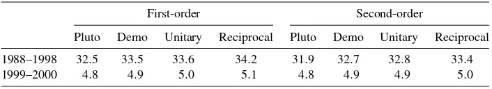
If preferences or budgets are heterogeneous across people (as they clearly are), then individual cost-of-living indexes are also heterogeneous. Thus, any social cost-of-cost-of-living index faces an aggregation problem. In this article, we provide a solution to this problem that we call a “common-scaling” social cost-of-living index (CS-SCOLI). In addition, we describe nonparametric methods for estimating such social cost-of-living indexes. As an application, we consider changes in the social cost-of-cost-of-living in the U.S. between 1988 and 2000.
KEY WORDS: Average derivatives; CPI; Demand; Inflation.
1. INTRODUCTION
“How has the cost-of-living changed?” is one of the first questions that policy makers and the public ask of economists. One reason is that a vast amount of public expenditure is tied to measured changes in the cost-of-living. For example, many public pensions are indexed to measures of the overall or “so-cial” cost-of-living. While economists have a well-developed theory of the cost-of-living for a person, they do not have a similarly well-developed theory for the cost-of-living for a soci-ety. If preferences and budgets are identical across people, then the cost-of-living index is identical across people and there is no problem in identifying the social cost-of-living index. How-ever, if preferences or budgets are heterogeneous across people (as they clearly are), then different people experience different changes in the cost-of-living, which must be somehow aggre-gated into a cost-of-living index for the society as a whole. In this article we present a new class of social cost-of-living in-dexes. These indexes aggregate the cost-of-living indexes of heterogeneous individuals. In addition, we describe nonpara-metric methods for estimating these and other social cost-of-living indexes.
Most social cost-of-living indexes in use—such as the Con-sumer Price Index (CPI)—can be understood as aggregator functions of approximations of household cost-of-living in-dexes [see, e.g., Prais 1958 or Nicholson 1975, and espe-cially, Diewert’s (1998) overview]. The CPI is the expenditure-weighted average of first-order approximations of each house-hold’s cost-of-living index (COLI). It is troubling for at least three reasons. First, it has not been shown to have a welfare economic foundation for the case where agents are heteroge-neous. Second, the CPI uses an expenditure-weighted average, which down-weights the experience of poor households relative to rich households (and thus is sometimes called a “plutocratic” index). Finally, it uses only first-order approximations of each individual’s cost-of-living index, and thus ignores substitution effects.
Many researchers have used an alternative, called the “de-mocratic index,” equal to the arithmetic mean of household
COLI’s. In practice, a first-order approximation to this index is implemented (using only first-order approximations of each in-dividual’s cost-of-living index). Recent work includes Kokoski (2000), Crawford and Smith (2002), and Ley (2002, 2005). This alternative approach addresses our second concern, but not the other two. Pollak (1981) offered a social cost-of-living index that is explicitly grounded in a welfare economic problem. His solution is elegant, but as we shall elaborate in the following, it can be difficult to compute and interpret. In particular, the thought experiment corresponding to his index involves differ-ent income adjustmdiffer-ents for differdiffer-ent individuals. However, in practice, we use social cost-of-living indexes to make equipro-portionate adjustments to incomes, for example, in adjusting public pension levels.
We provide a simple, easy-to-interpret, easy-to-estimate so-lution to the problem of aggregating different changes in the cost-of-living into a social cost-of-living index. For an individ-ual, the change in the cost-of-living is the answer to a question: what scaling of expenditure will hold utility constant over a price change? Our new social cost-of-living index is the answer to the following question. What single scaling to everyone’s ex-penditure will hold social welfare constant over a price change? We call this the “common-scaling” social cost-of-living in-dex (CS-SCOLI). It has the following advantages. First, the “common-scaling” aspect of our index is attractive both be-cause it is analogous to the individual cost-of-living index and because it corresponds directly to the feasible policy uses of a social cost-of-living index (i.e., equiproportionate income ad-justments). Second, our social cost-of-living index has social welfare foundations and allows the investigator to easily choose the “welfare weight” placed on rich and poor households. Third, nonparametric first-order approximations of the CS-SCOLI are easy-to-implement with commonly available commodity price
© 2010American Statistical Association Journal of Business & Economic Statistics October 2010, Vol. 28, No. 4 DOI:10.1198/jbes.2009.06139
523
and consumer expenditure data. Fourth, it is possible to com-pute nonparametric second-order approximations that capture substitution effects. Finally, the CS-SCOLI nests the plutocratic index and an object that is quite similar to the democratic index. The rest of the article proceeds as follows. In the next sec-tion we formally define the CS-SCOLI and compare it to other social cost-of-living indexes. In Section3 we derive the order approximation to the CS-SCOLI and compare its first-order approximation to that of other social-cost-of living in-dexes. Section4develops second-order approximations to the CS-SCOLI, the plutocratic SCOLI, and the democratic SCOLI. It also describes nonparametric methods for estimating them. Our method relies on nonparametric estimates of average deriv-atives and is similar in spirit to that proposed by Deaton and Ng (1998). In the presence of unobserved preference heterogeneity, estimation of the second-order terms in the approximations to plutocratic SCOLI and the democratic SCOLI faces a problem posed by Lewbel (2001). Another contribution of this article is that we offer a solution to this problem. Section5 contains a small Monte Carlo study, in which we show that both welfare weights and second-order effects might matter. In Section6, we present an empirical illustration that considers changes in the social cost-of-living in the U.S. between 1988 and 2000. We find that both the weighting of rich and poor households and the incorporation of second-order effects have only modest im-pacts on our assessment of changes in the social cost-of-living. Section7concludes.
2. THEORY
2.1 Individual Cost-of-Living Index
The standard theory of the cost-of-living for a person is as follows. Letu=V(p,x,z)be the indirect utility function that gives the utility level for an individual living in a household with aTvector of demographic or other characteristicsz, total expenditurex, and facing the price vectorp= [p1, . . . ,pM]. Let
x=C(p,u,z)be the cost function, which is the inverse ofV
overx. Leti=1, . . . ,Nindex individuals, each of whom lives in a household with one or more members. For each individual, the number ni gives the number of members in that person’s household. Each individual has an expenditure levelxiequal to the total expenditure of that individual’s household.
Many calculations are done at the household, rather than the individual, level. For household-level calculations, leth=
1, . . . ,Hindex households, letxhbe the total expenditure,nhbe the number of members, andzhbe the characteristics of house-holdh. Note thatxh=xi(becausexiis the total expenditure of the household to which individualibelongs), so that, for exam-pleHh=1xh=Ni=1xi/ni.For simplicity, we consider environ-ments where expenditure levels and characteristics vary across households, but not within households, and where price vectors are common across all individuals/households at a point in time. Thus, we assume that all members of a given household attain the same utility level, and consequently, have the same cost-of-living index. Addressing intrahousehold variation in expendi-ture, and hence welfare, would be an interesting extension, but is beyond the scope of the current article.
We define the individual’s cost-of-living index (COLI), π(p,p,x,z), as the scaling to expenditurexthat equates util-ity between a reference price vector,p, and a different price vector,p. Formally,
V(p,x,z)=V(p, π(p,p,x,z)x,z), (1)
forπ. This individual COLI function over the pair of price vec-torspandpis defined for any expenditure level,x, including the actual expenditure of the household when facingporp.
Letxi be the expenditure level of person iwhen facing the reference price vector (typically observed in the data). Letui be the utility level of personiwhen facing the reference price vector:ui=V(p,xi,zi). We denote the individual’s COLI eval-uated at reference expenditures,xi, for the price change from reference prices,p, to new prices,p, as
πi=π(p,p,xi,zi)=C(p,ui,zi)/xi. (2) For a household-level calculation, we note thatπi=πhfor alli in householdh. Although most previous work is motivated with household-level calculations, the welfarist framework that we employ below necessitates an individual-level analysis. Since all household members are identical, and thus have the same COLI, moving between these levels of analysis is straightfor-ward and amounts to reweighting.
2.2 The Common-Scaling Social Cost-of-Living Index
We propose a social cost-of-living index (SCOLI) that is sim-ilar in spirit to the individual COLI defined by Equation (1). Let the direct social welfare function s=W(u1, . . . ,uN)give the level of social welfare,s, corresponding to a vector of utilities,
u1, . . . ,uN. We define the common-scaling social cost-of-living index (CS-SCOLI),∗, as the single scaling of all expendi-tures that equates social welfare at the two different price vec-tors. This definition requires a reference expenditure vector. We take the reference expenditure vector to be the actual expen-diture vector when facing the reference price vector. Denoting
x1, . . . ,xNas the reference expenditure vector, we solve
W(V(p,x1,z1), . . . ,V(p,xN,zN))
=W(V(p, ∗x1,z1), . . . ,V(p, ∗xN,zN)), (3) for ∗=∗(p;p,x1, . . . ,xN,z1, . . . ,zN). Just as a person’s cost-of-living index is the scaling to her expenditure that holds her utility constant over a price change, the CS-SCOLI is the scaling toeveryone’sexpenditure that holds social welfare con-stant over a price change. Clearly∗=1 at reference prices. However, at other prices it can be a complex implicit functional of the direct welfare function and indirect utility functions. Be-low, we will show cases in which the CS-SCOLI has an explicit representation and we show how to approximate it when it does not.
2.3 Previous Approaches to the Social Cost-of-Living
Since the COLI is different for individuals with differentx
andz, a social cost-of-living index must somehow aggregate
these individual COLI’s. The most commonly used SCOLI is the so-called plutocratic SCOLI,P, which may be defined as a weighted average of individual COLI’s given by
P= 1
H h=1xh
H
h=1
xhπh=
1
N i=1
xi
ni
N
i=1
xi
ni
πi. (4)
This SCOLI assigns the reference household expenditure weight to each household-specific COLI, or equivalently, as-signs the reference household per-capita expenditure weight to each person-specific COLI.
An alternative is the democratic SCOLI, D, which uses the unweighted average of household COLI’s instead of the expenditure-weighted average as follows:
D= 1
H
H
h=1 πh=
1
N i=1
1 ni
N
i=1 1
ni
πi. (5)
Here, individual COLI’s are weighted by the reciprocal of the number of household members. Both the plutocratic and de-mocratic SCOLI’s are weighted averages of individual COLI’s. The avoidance of expenditure weights in the weighted average is the great advantage of the democratic SCOLI (see, e.g., Ley 2005). We will show later in our discussion of first-order ap-proximations that the CS-SCOLI is approximately a weighted average of approximate individual COLI’s where the weights are determined by the curvature of the social welfare function in expenditures.
Although the plutocratic and democratic SCOLI’s are so-cial aggregator functions, neither has a welfare-economic ba-sis. Pollak (1981) offered a SCOLI that is explicitly grounded in a welfare economic problem. Define the indirect social cost function
M(p,s,z1, . . . ,zN)≡ min x1,...,xN
H
h=1
xh=
N
i=1
xi/ni,
st W(V(p,x1,z1), . . . ,V(p,xN,zN))≥s,
xi=xh ∀i∈h,
as the minimum total (across households) expenditure required to attain the level of social welfaresfor a population with char-acteristicsz1, . . . ,zN facing pricesp. Pollak’s proposal for a SCOLI is
M(p,p,s,z1, . . . ,zN)=
M(p,s,z1, . . . ,zN)
M(p,s,z1, . . . ,zN) ,
where s equals initial social welfare, new social welfare, or some other social welfare level. Here, the numerator is equal to the minimum total expenditure across all households required to get a welfare level ofswhen facing pricesp, and the denom-inator is the minimum total expenditure when facing reference pricesp.
Pollak’s is a very elegant solution to the aggregation problem, and it was implemented by Jorgenson and Slesnick (1983), Jor-genson (1990), and Slesnick (2001). Note that this procedure requires an optimization step in which the investigator deter-mines the optimal distribution of expenditure (income) in each price regime. With heterogeneous preferences across house-holds, this optimization can be hard. Moreover, if actual ex-penditure distributions are not optimal, comparisons of optimal
expenditure distributions may not be very compelling. Finally, individual adjustments to expenditure may not correspond to feasible uses of a social cost-of-living index.
Let s=W(V(p,x1,z1), . . . ,V(p,xN,zN)) be the reference level of social welfare attained if households have reference ex-penditures x1, . . . ,xN, characteristicsz1, . . . ,zN, and face the reference price vectorp. If the program defining Pollak’s index is evaluated at this level of welfare, then the CS-SCOLI can be understood as the solution to Pollak’s program subject to the additional constraint that expenditures must be proportional to the reference expenditure vectorx1, . . . ,xN:
M(p,s,z1, . . . ,zN)≡ min x1,...,xN
N
i=1
xi/ni,
st W(V(p,x1,z1), . . . ,V(p,xN,zN))≥s,
xi=λxi ∀i,
xi=xh ∀i∈h.
One can see by inspection that the CS-SCOLI is equal to the factor of proportionality:∗=λ.This restriction to Pollak’s program was independently proposed by Fisher (2005) and we discuss his results below. The “common-scaling” restriction is attractive. It corresponds directly to the feasible policy uses of a social cost-of-living index (i.e., equiproportionate income ad-justments). In addition, it constrains us to work with actual, rather than optimal, income distributions.
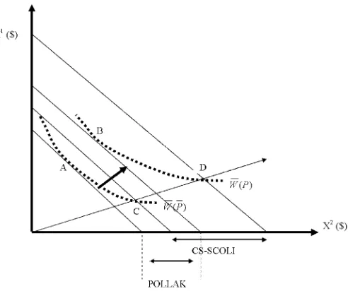
The relationship between the CS-SCOLI and Pollak’s pro-gram is illustrated in Figure1. The axes measure the total ex-penditure of two individuals. The straight lines running diago-nally down and to the right are social isocost lines. (If all house-holds are of the same size, these have slope−1.) The point C
indicates the initial expenditure distribution.
The curved dotted lines are level sets of the social welfare function (SWF). At the initial expenditure distribution (X) indi-cated by pointCand at the initial (reference) prices (P), social welfareW results. This level of social welfare can be achieved
Figure 1. The CS-SCOLI and Pollak’s SCOLI.
at minimum social cost at pointA (at a point of tangency be-tween a social isocost line and the level set of the SWF corre-sponding to W). ThusA represents the “optimal” expenditure distribution.
A change in prices (fromPtoP) shifts the level set of the SWF in expenditure space.W is now achieved with minimum social cost at pointB. The Pollak SCOLI is the ratio of the social cost ofBto the social cost ofA.
The ray from the origin indicates equiproportionate scalings of the original expenditure distribution. The pointDindicates whereWcan be achieved (given new pricesP) with an equipro-portionate scaling of budgets. This is the point where the ray from the origin intersects the level set labeledW(P). The CS-SCOLI is the ratio of the social cost ofDto the social cost ofC. The comparison ofAandBinvoked by Pollak’s SCOLI is a comparison of two unobserved, optimal, distributions. The in-come adjustments relating them are individual-specific. In con-trast, the comparison of C andD invoked by the CS-SCOLI is a comparison of an observed distribution, which may not be optimal, and a different distribution yielding the same welfare, which also may not be optimal. The income adjustments relat-ing them, though, are common to all people. The equipropor-tionate nature of the CS-SCOLI makes it a reasonable candi-date for policy purposes: most public policy applies the same cost-of-living adjustments to a large group of people.
2.4 Some Special Cases of the CS-SCOLI
The CS-SCOLI given by Equation (3) is expressed as an im-plicit function. In some cases, the CS-SCOLI may be expressed explicitly. The proposition below shows the explicit representa-tion of the CS-SCOLI for a few interesting cases. Our first case puts no restrictions on the welfare function, but requires identi-cally homothetic utility. The second case allows for nonhomo-thetic utility via the Price-Independent Generalized-Linearity (PIGL) structure (see Muellbauer1976for discussion), but is restricted to utilitarian welfare. The third case allows for nonu-tilitarian welfare via theS-Gini structure (see Donaldson and Weymark1980) and invokes a somewhat restricted form of non-homothetic PIGL utility. Throughout we assume that individu-als with the samezhave the same preferences.
Proposition 1. Let h(t) be monotonically increasing in t.
Leta(p,z)be homogeneous of degree 0 inp, andb(p,z)and
c(p)be homogeneous of degree 1 inp. Let d(z)be an arbi-trary function of z. Consider the PIGL indirect utility func-tion defined byV(p,x,z)=a(p,z)+(b(px,z))θ/θforθ=0 and
V(p,x,z)=a(p,z)[lnx−lnb(p,z)]forθ=0, with associated cost functionC(p,u,z)=b(p,z)θ1/θ(u−a(p,z))1/θ forθ=0 and lnC(p,u,z)=a(pu,z)+lnb(p,z)forθ=0.
1. If indirect utility is identically homothetic with V(p,x, z)=h(b(p)xd(z))and the direct welfare function depends only on the utility vector (i.e., is “welfarist”), then the CS-SCOLI is given by
∗(p;·)=b(p)
b(p).
2. If indirect utility is PIGL and the direct welfare function is utilitarian, whereW(·)=Ni=1ui, then the CS-SCOLI is given
3. If indirect utility is PIGL with a independent of z
[a(p,z)=a(p)] andbmultiplicatively separable withb(p,z)=
c(p)d(z), and the direct welfare function is a weighted sum of utilities, whereW(·)=Ni=1giui, withS-Gini weightsgi that sum to 1 and depend only on personi’s position in the distribu-tion of utilities, then the CS-SCOLI is given by
∗(p; ·)= and h is monotonic in xi, this is a unique solution. Cases 2 and 3: SubstituteW(·)andV(p,x,z)into Equation (3) and re-arrange to get explicit formulas for ∗. Note that in Case 3, the restrictions onaandbensure that, given the distribution of expenditures, the distribution of utilities—and therefore the set of weightsgi—does not depend on prices.
In Cases 2 and 3, the direct welfare function is (piecewise) linear and indirect utility is linear in a function of expenditure at each price vector. This ensures that both sides of the implicit definition of the CS-SCOLI given by Equation (3) are linear in a function of∗, so that solving for∗is straightforward. The linearity of the solutions (combined with the concavity of indi-vidual cost in prices) also implies that the CS-SCOLI is concave in prices for these cases.
In Case 1, the direct welfare function may be nonlinear, but since preferences are homothetic, this nonlinearity drops out of the expression for∗. That is, since this homothetic indi-rect utility function implies individual COLI’s are independent of expenditure and demographics, the CS-SCOLI is equal to
this (common) individual COLI regardless of the inequality-aversion of the social welfare function.
We note that the PIGL functional form for indirect utility ex-ploited in the proposition was also used by Muellbauer (1974) in his exploration of the political economy of price indexes. However, his focus was on how a common price index might be redistributive, whereas ours is on the welfare basis of a po-tential common price index.
Two examples of Case 2 of Proposition1are of specific inter-est. Given PIGL utility, one may substitute the individual COLI, πi, into the expression for the CS-SCOLI. If θ=1, then the marginal utility of money is constant and preferences are quasi-homothetic so that commodity demands are linear in expendi-ture. Ifb is multiplicatively separable withb(p,z)=c(p)d(z) and d(z)=ni, then costs are proportional to the number of household members and independent of all other demographic characteristics. With these restrictions, some (tedious) algebra reveals that the CS-SCOLI is given by the plutocratic SCOLI:
∗(p;p,x1, . . . ,xN,z1, . . . ,zN)=
Thus, with quasihomothetic utility and costs depending linearly on household size, the CS-SCOLI coincides with the plutocratic SCOLI.
Ifθ=0, then the marginal utility of log-money is a constant and preferences are PIGLOG with commodity budget shares that are linear in the log of expenditure. Ifbis multiplicatively separable withb(p,z)=c(p)d(z), then the CS-SCOLI is given by theunitary SCOLI defined as the geometric mean of indi-vidual COLI’s:
The unitary social cost-of-living index gives the same weight to everyone’s individual cost-of-living index, so it is similar in spirit to the democratic SCOLI. However, the unitary SCOLI is a geometric rather than an arithmetic mean.
3. FIRST–ORDER APPROXIMATION
3.1 First-Order Approximation of the CS-SCOLI
Consider the approximation of the cost-of-living index for an individual household. Letwbe theM vector of budget-shares, with a subscript for household or individual. Define the com-pensated (Hicksian) budget-share vector-function,ω(p,u,z), to give the budget-share vector for a person with utilityuand char-acteristicszfacing pricesp. Note that, by Shephard’s Lemma, w=ω(p,u,z)= ∇lnplnC(p,u,z). We typically invoke Shep-hard’s Lemma at the reference price vector and utility value. Define the uncompensated (Marshallian) budget-share vector-functions,w(p,x,z), to give the budget-share vector for a per-son with household expenditurexand characteristicszfacing pricesp.
We assume knowledge of the reference, or initial, price vec-tor,p, and of micro-data on budget-shares, expenditures, and demographics,{wi,xi,zi}Ni=1, for individuals facing this initial price vector. We assume knowledge only of price data,p, in the
nonreference, or final, period. We note thatzidoes not have an overbar because it is assumed to be invariant for an individual. In this article, the reference price vector is taken to be the ini-tial price vector, so that our approach is similar in spirit to the Laspeyres index for an individual COLI. It is possible to refor-mulate our concept with the reference price vector given by the final price vector, which is similar in spirit to the Paasche for-mulation. Since our approximation strategies require informa-tion on budget shares in the reference period, we feel that the Laspeyres approach is more useful. Donaldson and Pendakur (2009) considered the question of when these two indexes are equivalent.
The first-order approximation of πi aroundp for a person with expenditure xi and demographics zi is the well known Laspeyres index for the individual,πiL,
πi≈πiL≡1+dp′wi, (6) wheredp≡ [p1−p1
p1 , . . . ,
pM−pM
pM ]is theMvector of
proportion-ate price changes. This type of approximation requires micro-level information only from the reference period, so it is easily implemented with real-world data. For example, Crawford and Smith (2002) evaluated this approximation to the household-level COLI for a sample of UK households between 1976 and 2000 and find great heterogeneity in (approximate) COLI’s across households.
A first-order approximation to the plutocratic SCOLI is com-monly computed by statistical agencies for several reasons. For example, the linearity of the approximation makes it decompos-able by groups. In addition, it may be interpreted in terms of an “aggregate consumer” whose behavior is described by that of the economy as a whole. From our point of view, its key feature is that it is computable using only aggregate data. In particular, sinceP is linear inπi, we may substitute Equation (6) into Equation (4) to obtain a first-order approximation ofP:
P≈N1 aggregate reference budget-share vector for the population. This methodology is used by the Bureau of Labor Statistics to compute the CPI.
Crawford and Smith (2002) estimated the first-order approx-imation ofD, hold-level average budget-share vector (rather than the aggre-gate budget-share vector). They find in their study of UK data that the approximate democratic SCOLI shows slightly less in-flation than does the approximate plutocratic SCOLI.
Defining the weights
we may write the first-order approximations of the plutocratic and democratic indexes as
m≈ N
i=1 φimπiL,
form=P,D. It turns out that the first-order approximation of the CS-SCOLI also takes the form of a weighted average of individual Laspeyres indexes.
An approximation of the CS-SCOLI, ∗, around p may be obtained via the implicit function theorem. Let (·) de-note the reference values of function arguments and let over-bars denote the values of functions evaluated at their ref-erence arguments. Thus, we denote refref-erence utility levels and functions as ui =V(·)≡V(p,xi,zi), and the reference welfare level and function as s=W(·)≡W(u1, . . . ,uN)=
W(V(p,x1,z1), . . . ,V(p,xN,zN)). The equation defining the CS-SCOLI may be rewritten as
s=W V(p, ∗(p)x1,z1), . . . ,V(p, ∗(p)xN,zN), where∗(p)=∗(p;p,x1, . . . ,xN,z1, . . . ,zN)suppresses the dependence of the CS-SCOLI on the reference price and expen-diture vectors and demographic characteristics vectors. Here, we emphasize that∗(p)depends onpas a variable. Applica-tion of the implicit funcApplica-tion theorem yields
∇p∗(p)= −
N
i=1∇uiW(·)∇pV(p, ∗(p)xi,zi)
N
i=1∇uiW(·)∇xiV(p, ∗(p)xi,zi)xi
. (11)
Define the normalized proportionate welfare weight for person
i’s household expenditure as
φi(p)=φi(p;p,x1, . . . ,xN,z1, . . . ,zN) ≡ ∇uiW(·)∇xiV(p, ∗(p)xi,zi)xi
N
i=1∇uiW(·)∇xiV(p, ∗(p)xi,zi)xi
, (12)
and let
φi=φi(p)= ∇
uiW(·)∇xiV(p,xi,zi)xi
N
i=1∇uiW(·)∇xiV(p,xi,zi)xi
(13)
= N∇uiW(·)∇lnxiV(p,xi,zi) i=1∇uiW(·)∇lnxiV(p,xi,zi)
(14)
be the reference value of the normalized proportionate welfare weight for personi’s household expenditure. Sinceφi=φi(p) is evaluated at reference prices, and since∗(p)=1 at refer-ence prices,∗(p)drops out of the expression forφi. Again, we suppress the dependence ofφion(p,x1, . . . ,xN,z1, . . . ,zN) be-causeφi(p)only depends onpas a variable. A welfare weight is usually defined as the response of social welfare to individual expenditure,∇uiW(ui, . . . ,uN)∇xiV(p,xi,zi). For convenience,
we use aproportionate welfare weight, which multiplies this quantity by expenditure, and gives the response of welfare to a proportionate change in personi’s household expenditure. It
isnormalizedto sum to 1. Finally, it is areferenceweight
be-cause it evaluated at the reference price and expenditure vec-tors. The following proposition shows the first-order approxi-mation of∗.
Proposition 2. Given the normalized reference
proportion-ate welfare weights φi given by Equations (12) and (13) and reference budget shares wi, a first-order approximation of the
CS-SCOLI∗is
∗≈ N
i=1
φiπiL, (15)
or, equivalently,
∗≈1+dp′w, (16)
wheredp≡[p1−p1 p1 , . . . ,
pM−pM
pM ]is theM vector of proportion-ate price changes andw≡Ni=1φiwiis the weighted-average reference budget-share vector.
Proof. Let ∗(·) denote ∗(p;p,x1, . . . ,xN,z1, . . . ,zN).
Using the first-derivative of∗(·)given by Equation (11) and the fact that∗(p;p,x1, . . . ,xN,z1, . . . ,zN)=1, a first-order approximation of∗(p;p,x1, . . . ,xN,z1, . . . ,zN)is given by
∗(p;p,x1, . . . ,xN,z1, . . . ,zN) =1+(p−p)′∇p∗(·)
=1−(p−p)′
N
i=1∇uiW(·)∇pV(p,xi,zi)
N
i=1∇uiW(·)∇xiV(p,xi,zi)xi
.
Substituting in dp and the logarithmic form of Roy’s Iden-tity evaluated at reference prices and expenditures, wi = −∇lnpV(p,xi,zi)/∇lnxV(p,xi,zi), gives the approximation in terms of reference budget shareswi:
∗≈1+dp′ N
i=1∇uiW(·)∇xiV(p,xi,zi)xiwi
N
i=1∇uiW(·)∇xiV(p,xi,zi)xi
.
Substituting in the welfare weights Equation (12) yields Equa-tion (16).
3.2 Relationship to First-Order Approximations to Other SCOLI’s
In Section2.4we give conditions under which the CS-SCOLI and the plutocratic SCOLI coincide. Of course, when the exact indexes coincide, their first-order approximations coincide as well. The first-order approximation of the CS-SCOLI, Equa-tion (15), coincides with that of the democratic SCOLI if and only if
φi=N1/ni i=11/ni
, (17)
for alli=1, . . . ,N. This will obtain if welfare is utilitarian and indirect utility is PIGLOG withV(p,x,z)=a(p)+b(np)
i lnxi.
This indirect utility function corresponds to the widely used Almost Ideal demand system combined with constant marginal utility of log-money. Almost Ideal utility implies budget shares that are linear in the log of expenditure, a restriction that is not typically satisfied in real-world data (see, e.g., Banks, Blundell, and Lewbel1997). Here, the marginal social value of utility is a constant and the marginal utility of money for an individual is declining. (We note that this incorporation of household size is hard to interpret; the more common strategy in applied con-sumer demand or inequality measurement will be to deflatexi by a function of a weakly concave function ofni, rather than to deflate lnxibyni.)
Computationally, the expression in terms of weighted aver-age budget shares is convenient. Of course, the welfare-weights, φi, are themselves functions of the price, expenditures, and demographics (evaluated at reference prices and expenditures, p,x1, . . . ,xN), so implementation requires this information and requires the full knowledge of the welfare weight function. Fur-ther, since welfare weights must be calculated by the researcher, they must not depend on any unobserved factors. Such knowl-edge is routinely assumed in empirical investigations of in-equality and poverty and is required for an empirical investi-gation of the CS-SCOLI as well.
First-order approximations are exact for infinitesimal price changes. Fisher (2005) showed the CS-SCOLI is equivalent to Pollack’s SCOLI (Mdefined earlier) for an infinitesimal price change if the initial distribution is optimal. This is because, due to an envelope result applied to the social optimization, the al-ready optimal income distribution need not be re-adjusted in the face of a tiny price change. Fisher, Pollack, and Diewert all noted that if the initial distribution is optimal, then the first-order approximations of Pollack’s SCOLI and the plutocratic SCOLI coincide. This is due to an envelope result applied to the individual cost minimizations.
The assumption that the initial distribution is socially opti-mal also allows us to bound Pollak’s SCOLI (M) for large price changes. Pollak (1980) defined the “Scitovsky-Laspeyres” SCOLI as the proportionate increase total expenditure required to keep all households on their reference indifference curve, and shows that if the reference distribution of expenditure is so-cially optimal, then the Scitovsky-Laspeyres SCOLI is an upper bound on M. A first-order approximation to the Scitovsky-Laspeyres SCOLI is the aggregate Scitovsky-Laspeyres index in Equa-tion (7). Diewert (2001) considered the analogous “Scitovsky-Paasche” SCOLI defined as the proportionate increase total expenditure required to keep all households on their final indif-ference curve, and showed that if the final distribution was so-cially optimal, then the Scitovsky-Paasche SCOLI was a lower bound on M. A first-order approximation of this SCOLI is given by the aggregate Paasche index.
First-order approximations of bounds to Pollak’s SCOLI are thus easily implemented, and while these bounds are, in prin-ciple, very useful, they apply only to the case where the initial (or final) distribution of household expenditure is socially opti-mal. In contrast, the first-order approximation to the CS-SCOLI given in Proposition2approximates the index itself, rather than bounds for it, and applies to expenditure distributions that may not be socially optimal.
As noted earlier, if the CS-SCOLI is given by one of the ex-plicit representations given in Proposition1, it is concave in prices. Consequently, the first-order approximation to the CS-SCOLI provides an upper bound to its value. This bounding result contrasts with the bounding results of Pollak and Diew-ert concerning Pollak’s SCOLI. Their bounds apply only when the initial (or final) distribution of expenditure is socially opti-mal. Our bound applies regardless of the optimality of the ex-penditure distribution if welfare and indirect utility satisfy the requirements of one of the cases.
4. SECOND–ORDER APPROXIMATION
In this section we derive second-order approximations to the plutocratic and democratic SCOLI’s and to the CS-SCOLI. We also discuss estimation of these approximations. The second-order terms in the approximations to the plutocratic and de-mocratic SCOLI’s involve weighted averages of compensated price effects (on demand). Compensated price effects are de-fined by the Slutsky equation and involve products of levels and expenditure derivatives of demand equations. Lewbel (2001) showed that such compensated price effects may be difficult to estimate in the presence of unobserved preference heterogene-ity. In the following, we provide a solution to this problem, so that second-order approximations of the Plutocratic and Demo-cratic SCOLI’s may be estimated nonparametrically.
The second-order term in an approximation to the CS-SCOLI involves average uncompensated price effects, which do not involve products of levels and derivatives of demand equa-tions. These average uncompensated price effects may be esti-mated directly from data on budget shares, prices, total expen-diture, and demographics using standard nonparametric meth-ods (following, for example, Deaton and Ng1998). However, the second-order approximation to the CS-SCOLI brings a dif-ferent problem. As we shall show, it involves a term that is the response of the welfare weight functions to price changes. This cannot be estimated from demand data. We provide a propo-sition showing conditions under which this trailing term is ex-actly zero, and in the following section, we present a Monte Carlo study, one goal of which is to assess the likely size of this trailing term under a range of different assumptions. We begin with the plutocratic and democratic SCOLI’s.
4.1 Plutocratic and Democratic SCOLI’s
DefineWi≡wiw′i, and diag(wi)as a diagonal matrix with wi on the main diagonal. Define the matrix of compensated budget-share semielasticities asŴ(p,u,z)≡ ∇lnp′ω(p,u,z)=
∇lnp′w(p,x,z)+ ∇lnxw(p,x,z)w(p,x,z)′by the Slutsky theo-rem (that is, the chain rule). The second-order approximation of an individual COLI evaluated at reference prices and expendi-ture is given by
πi≈πiL+πiS, (18)
where
πiS=12dp′[Wi−diag(wi)+ ∇lnp′w(p,xi,zi) + ∇lnxw(p,xi,zi)w(p,xi,zi)′]dp =12dp′[Wi−diag(wi)+Ŵi]dp, where
Ŵi≡ ∇lnp′ω(p,ui,zi)
= ∇lnp′w(p,xi,zi)+ ∇lnxw(p,xi,zi)w(p,xi,zi)′ is the matrix of compensated budget-share price semielastici-ties evaluated at reference prices and utility (expenditure). The second-order term πiS is a quadratic form in the Slutsky ma-trix of substitution terms (expressed in budget-share form) and captures substitution effects in demand and savings from sub-stitution in the cost-of-living. Von Haefen (2000) showed how
the budget-share form is related to the more familiar quantity form of the Slutsky matrix.
Before considering the CS-SCOLI, which is defined implic-itly, it is instructive to consider the plutocratic and democratic indexes. Since both the plutocratic and democratic indexes are weighted averages of individual COLI’s [given by Equations (4) and (5), respectively], the second-order approximations of these indexes are the corresponding weighted averages of Equa-tion (18):
m≈ N
i=1
φim(πiL+πiS),
form=P,Dand whereφiPandφiDare given by Equations (9) and (10), respectively.
Estimates of these second-order approximations use weights φim (which depend on reference expenditures, xi and house-hold sizes,ni) plus budget shares,wi, and compensated semi-elasticities,Ŵi. All but the last are observable, and in the ab-sence of unobserved preference heterogeneity, the compensated semielasticities may be estimated nonparametrically using data on characteristics, budget shares, prices, and expenditures. Of course, consumption panel data would be appropriate, but re-peated cross-section data will also suffice. The nonparametric estimator of the compensated semielasticity matrix for an indi-vidual facing(p,xi,zi)is
Ŵi=∇lnp′w(p,xi,zi)+∇lnxw(p,xi,zi)wi′, (19)
where∇lnp′w(p,xi,zi)and∇lnxw(p,xi,zi)are nonparametric estimates of∇lnp′w(p,xi,zi)and∇lnxw(p,xi,zi), respectively (see Lewbel 2001). Since the convergence rate of this object is dominated by the derivatives, the estimators forPandD behave as (weighted) average derivative estimators.
In the presence of unobserved preference heterogeneity, Lewbel (2001) showed that the above estimator for Ŵi may be inconsistent. The basic problem is that unobserved pref-erence parameters may affect both ∇lnxw(p,xi,zi) and wi, which can induce covariance between them. In this case,
∇lnxw(p,xi,zi)w′iwill not equal the expectation of∇lnxw(p,xi, zi)w′i, but will instead have a matrix of bias terms equal to the unobserved covariance between ∇lnxw(p,xi,zi) and wi. The following proposition gives an estimator forŴithat exploits the restriction of Slutsky symmetry to get around Lewbel’s prob-lem.
Proposition 3. Taking Slutsky symmetry as a maintained
as-sumption for individual demands and assuming that unobserved preference heterogeneity is independent of p,x,z(which im-plies conditional exogeneity), thenŴimay be estimated consis-tently with
Ŵi≡12 ∇lnp′w(p,xi,zi)+ ∇lnp′w(p,xi,zi)
′
+∇lnx[w(p,xi,zi)w(p,xi,zi)′]
, (20)
where ∇lnp′w(p,xi,zi) is a consistent estimator for the un-compensated price semielasticity matrix of budget shares and
∇lnx[w(p,xi,zi)w(p,xi,zi)′]is a consistent matrix-valued esti-mator for the the expenditure semielasticity of the outer product
of budget-share vector-functions. Any of the standard nonpara-metric estimators (including, for example, local linear deriva-tive estimators) provides a consistent estimator for these ob-jects.
Proof. Given Slutsky symmetry,Ŵ(p,u,z)=Ŵ(p,u,z)′, so
that
∇lnp′w(p,x,z)+ ∇lnxw(p,x,z)w(p,x,z)′
=(∇lnp′w(p,x,z))′+w(p,x,z)∇lnxw(p,x,z)′, which implies that
2Ŵ(p,u,z)= ∇lnp′w(p,x,z)+ ∇lnxw(p,x,z)w(p,x,z)′ +(∇lnp′w(p,x,z))′+w(p,x,z)∇lnxw(p,x,z)′. Thus, we have
Ŵ(p,u,z)=21 ∇lnp′w(p,x,z)+ ∇lnxw(p,x,z)w(p,x,z)′ +(∇lnp′w(p,x,z))′+w(p,x,z)∇lnxw(p,x,z)′
,
and the symmetry-restricted estimated matrix of compensated semielasticities for a person i, may be written as in Equa-tion (20).
The intuition here is as follows. The troublesome term is
∇lnxw(p,xi,zi)w′i. Even if unobserved preference heterogene-ity parameters are independent ofp,x,z, there may be corre-lation between how such heterogeneity affects the slope and level of budget shares. Since we are interested in the product of those, such a correlation will manifest as bias. In contrast, under the maintained restriction of Slutsky symmetry, the ex-penditure derivative of the outer product of budget shares has the appropriate product inside it, so we can estimate it directly. Thus, it is the added restriction of Slutsky symmetry that allows us to avoid Lewbel’s problem.
Denoting the estimated value ofŴiasŴi[using either of the estimators given by Equations (19) or (20)], define the pluto-cratic and demopluto-cratic weighted average budget shares, outer-product of budget shares, and compensated semielasticity ma-trices as
wm= N
i=1 φimwi,
Wm= N
i=1 φimWi,
Ŵm= N
i=1 φimŴi,
for m=P,D. Given these objects, we can write the second-order approximations of the plutocratic and democratic indexes as
P≈1+dp′wP+12dp′[WP−diag(wP)+ŴP]dp, (21) D≈1+dp′wD+12dp′[WD−diag(wD)+ŴD]dp. (22)
4.2 CS-SCOLI
As with the Plutocratic and Democratic SCOLI’s, second-order approximation of the CS-SCOLI allows the researcher to account for substitution effects. However, unlike those SCOLI’s, the CS-SCOLI is not generally linear the individual COLI’s, which makes its approximation slightly more complex. In particular, the second-order approximation of the CS-SCOLI has an additional term, which accounts for changes in the wel-fare weights as prices change. The following proposition estab-lishes the second-order approximation of the CS-SCOLI:
Proposition 4. Given the normalized reference proportionate
welfare weights,φi, their local price responses,∇lnp′φi(p,x1, . . . ,xN,z1, . . . ,zN), reference budget shares,wi, and their price and expenditure derivatives, the second-order approximation of the CS-SCOLI∗is
∗≈1+dp′w+12dp′ww′−diag(w)
+∇lnp′w+∇lnxww′+
dp, (23)
where
w≡ N
i=1 φiwi,
∇lnp′w≡
N
i=1
φi∇lnp′w(p,xi,zi),
∇lnxw=
N
i=1
φi∇lnxw(p,xi,zi),
and
≡ N
i=1
φiwi∇lnp′lnφi(p,x1, . . . ,xN,z1, . . . ,zN).
Here, tildas (with no subscript i and no superscript) denote welfare-weighted averages.
Proof. See AppendixB.
The second-order approximation of the CS-SCOLI differs from a weighted average of second-order approximations of individual COLI’s in two ways. First, it contains products of weighted averages rather than weighted averages of products, for exampleww′ rather thanW. Second, it contains, which captures the response of the welfare weight functions to price changes. We note that if the CS-SCOLI is equal to the pluto-cratic SCOLI (for example, if welfare is utilitarian, the marginal utility of money is a constant and preferences are quasihomo-thetic), then the second-order approximation of the CS-SCOLI equals that given for the plutocratic SCOLI in Equation (21). In that case,ww′+∇lnxww′=W+∇lnxww′and=0(the first follows from the constant marginal propensities to consume un-der quasihomothetic preferences; we discuss the latter condi-tion in detail below).
For purposes of calculation and estimation, Equation (23) is convenient. The first three terms in this approximation are easily constructed from data given the welfare weightsφi. The weighted average budget shares,w, are computed directly from
the data and the welfare weights. The next two terms may be computed using the estimated weighted average derivatives,
∇lnp′wand∇lnxw. These objects may be estimated at efficient convergence rates using any of the standard average derivative estimators, including a weighted version of the score-type es-timator for the average of∇lnp′wproposed by Deaton and Ng (1998).
The trailing term of the approximation is driven by the price elasticity of the normalized proportionate reference welfare weights. If, at reference arguments, these welfare weights are highly elastic with respect to prices, then this term may po-tentially be large. Unfortunately, although applied researchers studying inequality were very willing to assume knowledge of welfare weights, our guess is that assuming knowledge of the elasticity of these weights with respect to prices will be less popular.
We propose to explore two ways to get a sense of the size of this trailing term. First, in the proposition below, we pro-vide some sets of sufficient conditions for this term to be ex-actly zero. Note that the trailing term may be written as=
N
i=1wi∇lnp′φi(p,x1, . . . ,xN,z1, . . . ,zN), which is the empiri-cal covariance between budget shares and the price semielastic-ities of the welfare weight functions (it is a covariance matrix, rather than just a moment matrix because the sum of ∇lnp′φi is zero by construction). The sufficient conditions we give in our proposition are sufficient conditions for uncorrelatedness, either by makingwithe same for alli=1, . . . ,Nor by making ∇ln′ plnφi(p)=0 for all i=1, . . . ,N. Identically homothetic preferences imply the former case. A welfare weight function that is independent of prices implies the latter. The cases in which we show that the trailing term is zero are very similar to the cases in which we show that the CS-SCOLI has an explicit representation. A second way we can assess the importance of the trailing term is via a Monte Carlo exercise. We show in the next section that in a plausible setting, the trailing term is very small.
Proposition 5. Define a(p,z),b(p,z),c(p),d(z), and h(t)
as in Proposition1. Define PIGL indirect utility as in Propo-sition 1: V(p,x,z)= a(p,z)+(b(px,z))θ/θ for θ = 0 and
V(p,x,z)=a(p,z)[lnx−lnb(p,z)] for θ =0. The trailing term in Equation (23) is exactly zero if any of the following sets of conditions hold:
1. Indirect utility is identically homothetic withV(p,x,z)=
h(c(p)xd(z)), and the direct welfare function depends only on the utility vector (i.e., is “welfarist”);
2. Indirect utility is PIGL withθ=0, andb is multiplica-tively separable whereb(p,z)=c(p)d(z), and the direct welfare function is utilitarian whereW(·)=Ni=1ui; 3. Indirect utility is PIGL with θ=0 (aka PIGLOG),a is
multiplicatively separable wherea(p,z)=c(p)d(z), and the direct welfare function is utilitarian where W(·)=
N i=1ui;
4. Indirect utility is PIGL,a is independent ofz[a(p,z)=
a(p)], b is multiplicatively separable where b(p,z)=
c(p)d(z), and the direct welfare function is a weighted sum of utilities where W(·)=iN=1giui, with S-Gini weightsgi which sum to 1 and depend only on person
i’s position in the distribution.
Proof. Case 1: With identically homothetic preferences, πi (and therefore dπi) is identical for all i=1, . . . ,N, and so is uncorrelated with dφi. Since Ni=1dφi =0, we have
N
i=1dπiLdφi=0. Cases 2, 3, and 4: See AppendixB.
These cases include reasonable combinations of welfare and indirect utility functions. For example, Case 2 includes the case where the direct welfare function is utilitarian with
W =Ni=1ui and indirect utility is PIGLOG [corresponding to the Almost Ideal demand system (Deaton and Muellbauer 1980)] with V(p,x,z)=a(p)[lnx−lnb(p,z)]. In this case, ∇uiW(·)=1 and∇lnxV(p,x,z)=a(p). Consequently, we have
φi(p,x1, . . . ,xN,z1, . . . ,zN)=1/N, which is obviously invari-ant to prices.
The uncorrelatedness required for the trailing term to be zero is clearly restrictive. However, we note two important fea-tures of our sufficient conditions. First, Cases 2 and 3 have PIGL indirect utility wherein preferences may be nonhomo-thetic. The PIGL class contains as cases both quasihomothetic preferences and PIGLOG preferences, both of which are com-monly used rank-2 demand systems. This result is slightly counterintuitive because many have shown (e.g., Banks, Blun-dell, and Lewbel1996) that standard welfare weights defined as∇uiW(ui, . . . ,uN)∇xiV(p,xi,zi)are independent of prices if
and only if V is quasihomothetic. This is because∇xiV is
in-dependent of prices if and only if V is affine in (a function of) expenditures. Quasihomotheticity of indirect utility implies marginal propensities to consume goods that are independent of expenditure for all goods, and is consequently an undesir-able restriction. However, since our normalized welfare weights have the population sum of welfare weights in the denomina-tor, we require a weaker restriction onV, namely that∇xiV is
multiplicatively separable into a function of prices only and a function of expenditure and demographics.
Second, Cases 1 and 3 allow for a direct welfare function that is averse to inequality in utilities. Although Case 1 requires identically homothetic preferences, Case 3, which covers the
S-Gini class of inequality-averse direct welfare functions (see Donaldson and Weymark 1980; Barrett and Pendakur 1995), does not require homothetic preferences.
This section develops a strategy to estimate second-order ap-proximations of various social cost-of-living indexes. As in the first-order approximation, our method does not require a para-metric model of consumer demand. Another similarity is that our nonparametric estimation strategy is robust to independent preference heterogeneity. However, in contrast to the first-order approximation case, our nonparametric estimation strategy may suffer from bias (endogeneity) if unobserved preference het-erogeneity is correlated with observables such as expenditure or demographics. Consequently, a second-order approximation may not be better than a first-order approximation.
5. MONTE CARLO EXPERIMENT
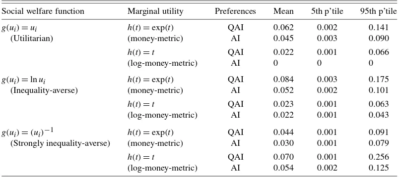
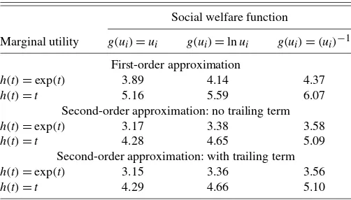
Here, we set up an experiment to establish two features of the CS-SCOLI in plausible environments: (1) the trailing term in the second-order approximation is small; and (2) both the welfare weights and the second-order approximation may affect the SCOLI in sizeable ways. To assess these for a given price
vector, we need to specify the distributions of expenditures and demographic characteristics and the structure of consumer pref-erences. For these, we use the data and empirical specification developed in Pendakur (2002). In addition, we need to spec-ify the social welfare function and consumer marginal utility of money. For these, we use utilitarian and inequality-averse so-cial welfare functions plus utility linear either in expenditure or the log of expenditure.
To mimic the data used by Pendakur (2002), we use a single demographic characteristic, the number of household members, and draw 1000 values of log-expenditure and the number of household members from independent standard normals with means of 4.54 and 2.17, respectively, and standard deviations of 0.65 and 1.31, respectively. The number of household members is discretized to 1,2,3, and so on.
For consumer preferences, we use the nine-good paramet-ric demand system estimated by Pendakur (2002) in which all households have a single demographic characteristic,z, equal to the number of household members and have quadratic almost ideal (QAI) indirect utility (see Banks, Blundell, and Lewbel 1997) given by
V(p,x,z)=k+h
lnx−lna(p,z)
b(p)+q(p)(lnx−lna(p,z))
,
whereh is monotonically increasing and k=4 is chosen to keepV positive in the simulation. We use the following func-tional forms fora,b, andq:
lna(p,z)=d0+dz+lnp′a+lnp′Dz
+12lnp′A0lnp+ 1
2lnp′Azlnpz, lnb(p)=lnp′b,
q(p)=lnp′q,
where all parameter values are taken from Pendakur (2002, table 3) andι′a=1, ι′b=ι′q=0, ι′D=ι′A0=ι′Az=0M, A0=A′0, andAz=A′z. For convenience, let the reference price vector bep=1M·100 and letd0= −ln 100. Thus, lna(p,z)= lnb(p)=q(p)=0. Engel curves are quadratic in the log of ex-penditure. However, ifqis set to0, then Engel curves are linear in the log of expenditure.
For this indirect utility function, utility at the reference price vector is given by
ui=V(p,xi,zi)=k+h(lnxi−dzi).
Consequently, the functionhdetermines the marginal utility of money. Ifh(t)=exp(t), then V(p,x,z)=k+x/exp(dzi), so that at a vector of unit prices, the marginal utility of money is constant (1/exp(dzi)). We refer to this case as “money-metric utility.” If, in contrast,h(t)=t, thenV(p,x,z)=k+lnx−dzi, and at a vector of unit prices, the marginal utility of a propor-tionate increase in money is constant. We refer to this case as “log-money-metric utility.”
For the social welfare function, we use the generalized utili-tarian form withW(u1, . . . ,uN)=Ni=1g(ui). This yields util-itarianism, which is neutral to inequality of utilities, ifg(ui)=
ui. It yields social welfare, which is somewhat averse to in-equality in utilities ifg(ui)=lnuiand strongly averse ifg(ui)= −(ui)−1. These welfare functions correspond to the mean of or-derr, or Atkinson, class of social welfare functions with social