Principle:
The magnetic field along the axis of wire loops and coils of different di-mensions is measured with a tesla-meter (Hall probe). The relationship between the maximum field strength and the dimensions is investigated and a comparison is made between the measured and the theoretical ef-fects of position.
Tasks:
1. To measure the magnetic flux density in the middle of various wire loops with the Hall probe and to investigate its dependence on the radius and number of turns.
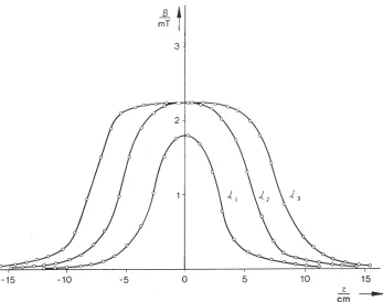
Curve of magnetic flux density (measured values) for coils with a constant density of turns n/l, coils radius R= 20 mm, lengths l1= 53 mm, l2= 105 mm and l3= 160 mm.
2. To determine the magnetic field constant 0.
3. To measure the magnetic flux density along the axis of long coils and compare it with theoretical values.
Experiment P2430215 with Cobra3
Experiment P2430201 with teslameter
Teslameter, digital 13610.93 1
Digital multimeter 07134.00 1
Induction coil, 300 turns, d= 40 mm 11006.01 1 1 Conductors, circular, set 06404.00 1 1
Hall probe, axial 13610.01 1 1
Power supply, universal 13500.93 1 1
Distributor 06024.00 1 1
Meter scale, demo, l= 1000 mm 03001.00 1 1
Barrel base -PASS- 02006.55 2 2
Support rod -PASS-, square, l= 250 mm 02025.55 1 1 Right angle clamp -PASS- 02040.55 1 2
G-clamp 02014.00 2 2
Lab jack, 200230 mm 02074.01 1 1 Reducing plug 4 mm/2 mm socket, 2 11620.27 1 1 Connecting cord, l= 500 mm, blue 07361.04 1 1 Connecting cord, l= 500 mm, red 07361.01 2 2
Bench clamp -PASS- 02010.00 1
Plate holder 02062.00 1
Silk thread, l= 200 m 02412.00 1
Weight holder 1 g 02407.00 1
Cobra3 Basic Unit 12150.00 1
Cobra3 Force/Tesla software 14515.61 1
Tesla measuring module 12109.00 1
Cobra3 Current sensor, 6 A 12126.00 1 Movement sensor with cable 12004.10 1 Adapter, BNC-socket/4mm plug pair 07542.27 2 Adapter, BNC socket - 4 mm plug 07542.20 1
What you need:
Complete Equipment Set, Manual on CD-ROM included
Magnetic field of a single coils /
Biot-Savart’s law
P24302 01/15
What you can learn about …
Wire loop Biot-Savart’s law Hall effect Magnetic field Induction
Magnetic flux density
Power supply, 12 V- 12151.99 1
RS232 cable 14602.00 1
PC, Windows® 95 or higher
Related topics
Wire loop, Biot-Savart’s law, Hall effect, magnetic field, induc-tion, magnetic flux density.
Principle
The magnetic field along the axis of wire loops and coils of dif-ferent dimensions is measured with a teslameter (Hall probe). The relationship between the maximum field strength and the dimensions is investigated and a comparison is made be-tween the measured and the theoretical effects of position.
Equipment
Induction coil, 300 turns, d= 40 mm 11006.01 1 Induction coil, 300 turns, d= 32 mm 11006.02 1 Induction coil, 300 turns, d= 25 mm 11006.03 1 Induction coil, 200 turns, d= 40 mm 11006.04 1 Induction coil, 100 turns, d= 40 mm 11006.05 1 Induction coil, 150 turns, d= 25 mm 11006.06 1 Induction coil, 75 turns, d= 25 mm 11006.07 1 Conductors, circular, set 06404.00 1 Teslameter, digital 13610.93 1 Hall probe, axial 13610.01 1 Power supply, universal 13500.93 1
Distributor 06024.00 1
Meter scale, demo, l= 1000 mm 03001.00 1 Digital multimeter 07134.00 1 Barrel base -PASS- 02006.55 2 Support rod -PASS-, square, l= 250 mm 02025.55 1
Right angle clamp -PASS- 02040.55 1
G-clamp 02014.00 2
Lab jack, 200230 mm 02074.01 1 Reducing plug 4 mm/2 mm socket, 2 11620.27 1 Connecting cord, l= 500 mm, blue 07361.04 1 Connecting cord, l= 500 mm, red 07361.01 2
Tasks
1. To measure the magnetic flux density in the middle of various wire loops with the Hall probe and to investigate its dependence on the radius and number of turns.
2. To determine the magnetic field constant m0.
3. To measure the magnetic flux density along the axis of long coils and compare it with theoretical values.
Set-up and procedure
Set up the experiment as shown in Fig. 1. Operate the power supply as a constant current source, setting the voltage to 18 V and the current to the desired value.
Measure the magnetic field strength of the coils (I= 1 A) along the z-axis with the Hall probe and plot the results on a graph. Make the measurements only at the centre of the circular con-ductors (I= 5 A). To eliminate interference fields and asym-metry in the experimental set-up, switch on the power and measure the relative change in the field. Reverse the current and measure the change again. The result is given by the aver-age of the measured values.
Theroy and evaluation
From Maxwell’s equation
(1)
wehre Kis a closed curve around area F, His the magnetic field strength, I is the current flowing through area F, and Dis the electric flux density, we obtain for direct currents , the magnetic flux law:
(2)
which, with the notations from Figs. 2, is written in the form of Biot-Savart’s law:
(3)
The vector dlis perpendicular to, and S and dH lie in the plane of the drawing, so that
(4)
dHcan be resolved into a radial dHrand an axial dHz
com-ponent.
The dHzcomponents have the same direction for all
conduc-tor elements dl
and the quantities are added; the dHr
com-ponents cancel one another out, in pairs.
Therefore,
Hr(z) = 0 (5)
and
H(z) =Hz(z) = (6)
along the axis of the wire loop, while the magnetic flux density
(7)
where µ0= 1.256610-6H/m is the magnetic field constant.
If there is a small number of identical loops close together, the magnetic flux density is obtained by multiplying by the num-ber of turns n.
the regression lines for the measured values in Figs. 3 and 4 give, for the number of turns, the following exponents Eand standard errors:
Fig. 2: Drawing for the calculation of the magnetic field along the axis of a wire loop.
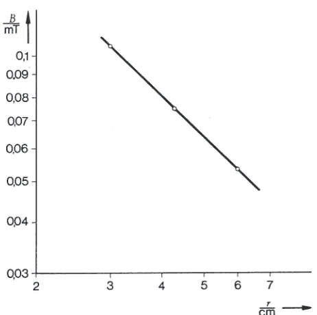
Fig. 3: Magnetic flux density at the centre of a coil with n turns, as a function of the number of turns (radius 6 cm, current 5 A).
and, for the radius (see equation (8))
E2= - 0.97 ± 0.02.
2. Using the measured values from Figs. 3 and 4, and equa-tion (8), we obtain the following average value for the magnet-ic field constant:
m0= (1.28 ± 0.01) 10-6H/m
3. To calculate the magnetic flux density of a uniformly wound coil of length land nturns, we multiply the magnetic flux den-sity of one loop by the denden-sity of turns n/land integrate over the coil length.
where
a= z+ l/2 and b= z– l/2.
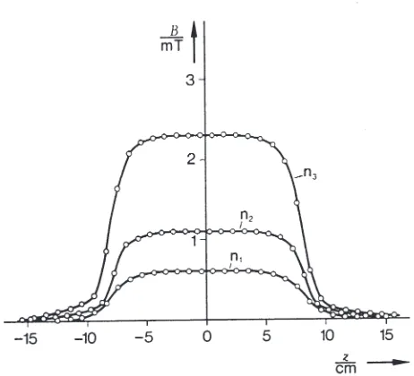
The proportional relationship between magnetic flux density B and number of turns nat constant length and radius is shown in Fig. 6. The effect of the length of the coil at constant radius with the density of turns n/lalso constant, is shown in Fig. 7.
Comparing the measured with the calculated values of the flux density at the centre of the coil,
gives:
B(0) mT
n measured calculated
75 160 13 0.59 0.58
150 160 13 1.10 1.16
300 160 13 2.30 2.32
100 53 20 1.81 1.89
200 105 20 2.23 2.24
300 160 20 2.23 2.29
300 160 16 2.31 2.31
R mm l
mm B 102 m0 · I · n
2l · aR 2
l
2b
12 , B 1z2 m0 · I · n
2l · a a 2R2
a2
b 2R2
b2b ,
Fig. 5: Magnetic flux density along the axis of a coil of length l = 162 mm, radius R = 16 mm and n = 300 turns; measured values (0) and theoretical curve (continuous line) in accordance with equation (9).