Artificial neural network-based harmonics extraction
algorithm for shunt active power filter control
Awan U. Krismanto and Abraham Lomi*
Department of Electrical Engineering, Institute of Technology Nasional Malang,
Jl. Raya Karanglo Km. 2, Malang 65143, Indonesia E-mail: [email protected]
E-mail: [email protected] *Corresponding author
Rusdy Hartungi
Department of Electrical Engineering, University of Central Lancashire, Preston, Lancashire, PR12HE, UK E-mail: [email protected]
Abstract: This paper presents a harmonics extraction algorithm using artificial neural network methods. The neural network algorithm was used due to the simpler calculation process compared with conventional method such as fast Fourier transform (FFT). Two types of neural network, i.e., multi-layer perceptron (MLP) and radial basis function (RBF) were employed to extract harmonics current component from its distorted wave current. Further, the extracted harmonics current was used as reference current for shunt active power filter (APF) control. This paper compared the performance of MLP and RBF for harmonics extraction. The advantages of RBF are simpler shape of the network and faster learning speed. Unfortunately, the RBF need to be trained recursively for various harmonics component. MLP can be used to extract various harmonics component in specific data range but need large number of data training hence slower training process.
Keywords: artificial neural network; ANN; radial basis function; RBF; multi-layer perceptron; MLP; harmonics extraction; shunt active power filter; SAPF.
Reference to this paper should be made as follows: Krismanto, A.U., Lomi, A. and Hartungi, R. (2012) ‘Artificial neural network-based harmonics extraction algorithm for shunt active power filter control’, Int. J. Power Electronics, Vol. 4, No. 3, pp.273–289.
Abraham Lomi received his BEng in Electrical Engineering from the Institute of Technology Nasional Malang, Indonesia in 1987, Master of Engineer in Electrical Engineering from the Institute of Technology Bandung, Indonesia in 1992 and Doctor of Engineering in Electric Power System Management from the Asian Institute of Technology, Thailand in 2000. He is currently Full-Professor at the Department of Electrical Engineering, Institute of Technology Nasional Malang and member of IEEE Power & Energy Society and Indonesian Institute of Engineers. His research interests include power system stability, power electronics, power quality and renewable energy.
Rusdy Hartungi received his MEng in Electrical Power Engineering from the Institute of Technology Bandung, Indonesia in 1992. In 1995–1996, he did 15 months post Master course at Swiss Federal Institute of Technology (ETHZ), Zurich/Switzerland. He obtained his PhD in Electrical Power and Energy Engineering from the Graz University of Technology, Austria in 2000. Prior to his appointment at The University of Central Lancashire – UK, he was working for many years as a Consulting Engineer in the UK. He is an active member of Institution of Electrical Engineer (IEE/IET) and Chartered Institution of Building Services Engineers (CIBSE). He is one of few UK chartered engineers. He has gained international recognition as International Professional Engineer (IntPE, UK) as well as European Engineer (Eur Ing).
1 Introduction
The significant increase of non-linear load usage such as power electronic equipment for voltage and current conversion, motor drives, switching power supplies and other electronics devices caused undesired impact to the power quality. The main effect of non-linear load usage is development of harmonics component contained in voltage and current waveform. The proliferation of harmonics causes voltage and current distortion, development of torque oscillation in electric machine, additional heating and losses in electrical equipment, malfunction of sensitive equipment and deteriorate power quality delivered to consumer in electrical power system (Chgangaroo et al., 1999).
Various methods have been introduced to overcome harmonics. In electrical drive for instance, the multilevel inverter triggered by unipolar PWM strategies could reduce the harmonics (Shanthi and Natarajan, 2010). Reduction of low order input current harmonics is also possible to be achieved by using switching modulation strategies (Babaei and Hosseini, 2010). Many compensators have been proposed to overcome the harmonics problem. Conventional method proposed for harmonics mitigation was passive filter tuned for specific harmonics order. Unfortunately, passive filter has some drawbacks such as generate parallel resonance with network impedance, poor flexibility for dynamics compensation of different harmonics component, aging and tuning problems and need larger dimension.
voltage regulation, voltage flicker reduction and voltage balanced improvement in three-phase system (Hassoun, 1995; Chen, 2003). Unfortunately, active filter have more complicated circuit and control algorithm.
Performance of active filter determined by the accuracy and precision of harmonics component extraction from distorted voltage and current waveform. Active filter control algorithms have been developing in order to obtain best performance to eliminate harmonics component from voltage and current waveform. Generally, fast Fourier transform (FFT) method used for harmonics extraction but its need more than one cycle data hence delay time will appear and may cause frequency deviation (Tey and So, 2002). Instantaneous p-q theory method has good performance, unfortunately it only suitable for three-phase system under balanced condition. Synchronous reference frame reference also suitable only for three-phase system and cause delays in filtering the DC value. Artificial intelligent algorithm widely used for signal processing. In this paper, two types neural network structure would be compared to get better performance for active filter control algorithm. The comparison between multi-layer perceptron (MLP) and radial basis function (RBF) can be seen through, number of layer and neuron, number of data needed for training, sum square error (SSE) value and time of training process. MATLAB Simulink will be used to simulate the shunt active power filter (SAPF) control algorithm based on neural network.
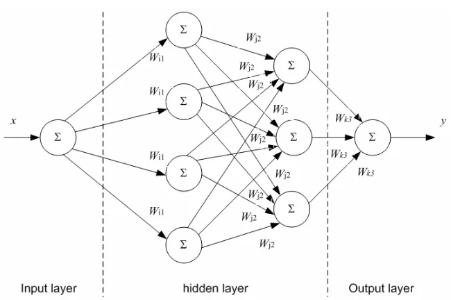
2 Multi-layer perceptron
MLP neural network is trained using Lavenberg-Marquardt back propagation (LMBP) algorithm. This algorithm used second order derivatives approximation without Hessian matrix calculation hence the training process become faster compared with conventional back propagation training algorithm in the way that it uses resulting derivatives for the weight updating. LMBP algorithm has forward and backward process. During the forward process it calculates the output error for the given dataset by fixing the weights. The weights are updated in backward process in order to obtain the desired output value.
The LMBP algorithm is described in the following steps (Tey and So, 2002): 1 Initialisation: all weight and biases are set to small random numbers that are
uniformly distributed.
2 Let the training set be {[p(1), t(1)], [p(2), t(2)], … [p(K), t(K)]}, where K represents the number of pattern in the training dataset, and p, t are input and desired output respectively. The input vector pattern p(n) is applied to input layer of sensory nodes and the desired output vector t(n) is presented to the output layer of computation nodes. The activation potentials vj(n) and function signals aj(n) of the network are
calculated by proceeding forward through the network, layer by layer. 0( ) ( ) for input layer
a k =p k (1)
(
)
1( ) 1 1 ( ) 1
0,1, , 1 and 1, 2, ,
l l l l l
a k f W a k b
l M k k
+ = + + + +
= … − = … (2)
( ) ( ) M( )
e k =t k −a k (3)
where ē is the error vector and k refers to training pattern presented to the network. Wl+1 is the weight matrix connecting lth and (l + 1)th layers and bl+1 is the bias vector for (l + 1)th layers.
3 The sum of squared error V over all the input is calculated using equation (4). 2
,
1 1 1
1 1
( ) ( )
2 2
M
S
K K
T
j k
k k j
V e k e k e
= = =
=
∑
=∑∑
(4)4 The error is passed in backward process and the weights are updated, layer by layer basis. In order to achieve this, the sensitivities or derivatives of the performance function with respect to weights are calculated. The gradient of V in terms of Jacobian can be presented by equation (5).
( ) ( )
T
V
J x e x x
∂ =
∂ (5)
1 1 1
1 2
2 2 2
1 2 1 2 ( ) ( ) ( ) ( ) ( ) ( ) ( ) ( ) ( ) ( ) C C
T T T
C
e x e x e x
x x x
e x e x e x
x x x
J x
e x e x e x
x x x
∂ ∂ ∂ ⎡ ⎤ ⎢ ∂ ∂ ∂ ⎥ ⎢ ⎥ ⎢∂ ∂ ∂ ⎥ ⎢ ∂ ∂ ∂ ⎥ = ⎢ ⎥ ⎢ ⎥ ⎢ ⎥ ∂ ∂ ∂ ⎢ ⎥ ⎢ ∂ ∂ ∂ ⎥ ⎣ ⎦ (6)
T in equation (6) is the product of number of the input/target pairs and the dimension of the neural network’s output vector SM and C is the total number of neural network
coefficients (weights and biases). The output error vector e x( ) can be represented as in equation (7).
[
1 2]
( ) ( ) ( ) T( )T
e x = e x e x e x (7)
The calculation of the above Jacobian matrix is the key step in LMBP algorithm. The Jacobian is a matrix of first order partial derivatives of a vector-valued function. It can be created by taking the partial derivatives of each output in respect to the each weight. In Lavenberg -Marquardt implementations, the Jacobian is approximated by using finite differences. For the neural networks, it can be computed very efficiently by using the chain rules of calculus and the first derivatives of the activation function. Hence, the derivative of equation (7) with respect to variable, which is one element of the Jacobian matrix, can be shown in equation (8).
(
)
, ( ) ( ) ( ) ( ) M M T T T T T CC C C
t k a k
e k a
J x
x x x
∂ −
∂ ∂
= = = −
∂ ∂ ∂ (8)
C
x can be wi jl,+1 or bil+1, where T = 1,2,…,T, c = 1,2, …, C, and l = 1, 2,…SM
(the number of neurons in input layer). For output neuron q, the net input (vqM) to the transfer function could be written as equation (9).
1 1 , 1 M S
M M M M
q q j j q j
v w a b
−
−
=
=
∑
+ (9)with aqM = f v( qM), we take the partial derivative with respect to wq jM, and bqM.
( )
( )
( )
1, , ,
M M
M M
q q
q q M M
q j
M M M M
q j q j q q j
f v f v
a v
f v a
w w v w
−
∂ ∂
∂ ∂
= = ⋅ =
∂ ∂ ∂ ∂ (10)
( )
M( )
M( )
M M
q q
q q M
q
M M M M
q q q q
f v f v
a v
f v
b b v b
∂ ∂
∂ ∂
= = ⋅ =
( qM)
f v is the derivative of activation function of the output layer with respect to the net input. Let σi ql,+1( )k be defined as one element of the sensitivity matrix σl+1( )k as shown in equation (12).
(
)
1
, 1 1
( ) ( )
( ) ( )
M M
q q
l
i q l l
i i
f v k
a k
v k v k
σ +
+ +
∂ ∂
= =
∂ ∂ (12)
In this algorithm, the sensitivity matrix is initialised at the output layer which given by first derivative of its transfer function.
(
( ))
M M M
F v k
σ = (13)
( )
M
v k is the vector of the net input to the transfer function and
( )
(
)
(
1 ( )) (
2 ( ))
(
M( ))
M M M M M
S
F v k =diag f v⎡⎣ k f v k …f v k ⎤⎦ (14)
After deriving all the above equations, the Jacobian matrix in (11) can be assembled using equations (10), (11), (13) and (14).
5 Finally the weights and biases are updated using equation (15) 1
( ) ( ) ( ) ( )
T T
x ⎡J x J x μI⎤− J x e x
Δ =⎣ + ⎦ (15)
μ in equation (15) us the step multiplier and e x( ) is the error vector. The equation approximates a gradient descent method if μ is very large. However, if μ is small, the equation becomes the Gauss-Newton method. As the second method is faster and more accurate near an error minimum, the aim is to shift toward the Gauss-Newton method as quickly as possible. Hence, μ is decreased after each successful step and increased only when a step increases the error. This means that if the sum of squared error is smaller than the previous step, μ is divided by a factor to decrease it, but it will be multiplied by a factor to increase if the sum of squared error is greater than that previous step.
For SAPF control, the MLP controller designed here as one input and one output with several hidden layers. The activation function is log-sigmoid in the hidden layers.
3 RBF neural network
with other areas of signal and pattern processing and other neural network architectures (Hassoun, 1995).
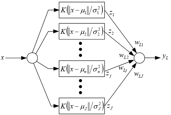
The RBF neural network has a feed forward structure consisting of a single hidden layer of J locally tuned units which are fully interconnected to an output layer of L linear units, as shown in Figure 2.
Figure 2 Typical structure of RBFNN
(
2)
1 1
σ
μ
−
x
K
(
2)
2 2
σ
μ
−
x
K
(
2)
n n
x
K
−
μ
σ
(
2)
J J
x
K
−
μ
σ
1
z
2
z
j
z
J
z
1
L
w
2
L
w
Lj
w
LJ
w
L
y
x
All hidden units simultaneously receive the n-dimensional real valued input vector x. The absence of hidden layer weights because the hidden unit outputs are not calculated using the weight-sum/sigmoid activation mechanism as MLP.
Each hidden-unit output zj is obtained by calculating the ‘closeness’ of the input x to
an n-dimensional parameter vector μj associated with the jth hidden unit.
2
( ) j
j
j
x
z x K μ
σ
⎛ − ⎞
= ⎜ ⎟
⎜ ⎟
⎝ ⎠
(16)
where K is a strictly positive radially-symmetric function (kernel) with a unique maximum at its ‘centre’ μj and which drops off rapidly to zero away from the centre. The
parameter σj is the ‘width’ of the receptive field in the input space for unit j. This implies
that zj has an appreciable value only when the ‘distance’ || x – μj || is smaller than the
width of σj. In this research, Gaussian function used as activation function for the hidden
units given as zj for j = 1,2,…,J, where
2
2 ( ) exp
2
j j
j
x
z x μ
σ
⎡ − ⎤
⎢ ⎥
= −
⎢ ⎥
⎣ ⎦
(17)
1
( ) ( )
J L Lj j
j
y x w z x
=
=
∑
(18)RBF networks are best suited for approximating continuous or piecewise continuous real valued mapping f: Rn→RL, where n is sufficiently small; these approximation problems include classification problems as a special case. According to equations (17) and (18), the RBF network may be viewed as approximating a desired function f(x) by superposition of non-orthogonal bell-shaped basis functions. The degree of accuracy can be controlled by three parameters: the number of basis functions used, their location, and their width. In fact, like feed forward neural networks with a single hidden layer of sigmoid units, it can be shown that RBF networks are universal approximator.
The training of RBF neural network is radically different from the classical training of standard feed forward neural network. In this case, there is no changing of weights with the use of gradient method aimed at function minimisation. In RBF neural networks with the chosen type of RBF, training resolves itself into selecting the centres and dimension of the functions and calculating the weight of the output neuron. The centre, distance scale and precise shape of the radial function are parameters of the model, all fixed if it is linear.
4 Shunt active power filter
SAPF connected in parallel with the non-linear load which has to be compensated. Basically APF worked to inject compensation current which have same magnitude but opposite phase with harmonics current contained in original distorted current. With current injection from SAPF the harmonics current component flowing in the system will be eliminated.
The operation of SAPF consists of two stages. First is detecting or sensing the harmonics current from the line and second is generating compensation current injecting to the line. The detected current used as input for ANN. The output of ANN is harmonics current component without fundamental component. The output of ANN will be used as reference signal compared with triangular signal to produce switching signal for voltage source inverter. Finally the current generated by inverter will be injected to the line as compensating current for harmonics mitigation. Control algorithm of SAPF based on ANN algorithm shown at Figure 3.
The switch used in the SAPF is IGBT. DC capacitor and the IGBT with anti parallel diode are used to indicate a SAPF built up from a voltage source converter (VSC) due to its high efficiency, low initial cost, and smaller physical size. There is no power supply at DC side of VSC, only an energy storage element (capacitor) is connected at the DC side of the converter. The reason is that the principal function of SAPF is to behave as a compensator (Akagi et al., 2007). We assume that the DC side capacitor has a constant voltage hence the dc voltage controller was not needed.
Figure 3 Control of SAPF-based on ANN algorithm (see online version for colours)
+ _
+ _
+ _
PI Controller
PI Controller
PI Controller PWM Switching
Generator
LPF
LPF
LPF Three Phase
AC Source
Nonlinear Load
Lsa
Lsb
Lsc
Isa
Isb
Isc
ILa
ILb
ILc
IhaIhb Ihc
ILa ILb ILb
Iha* Ihb* Ihc*
Harmonics Current Component Extraction
using Artificial Neural Network
5 Simulation results
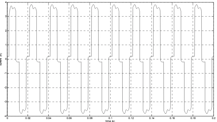
This research compared two ANN configurations types, i.e., MLP and RBF neural network for harmonics approximation function. The performance of neural network would be analysed through time of training process, network complicity, and value of SSE. To verify performance of proposed control algorithm, MATLAB Simulink used for simulating neural network based control model proposed for SAPF. The system was three-phase balanced system, 220 V, 50 Hz. Controlled thyristor rectifier which supplies resistive (500 Ω) and inductive (100 Ω and 0,1 H) loads used as non-linear load that would be compensated. The detected distorted currents were sampled at 10 kHz sampling frequency and 200 data in one cycle were taken as training data for the ANN. The distorted current from rectifier with resistive and inductive load can be seen at Figures 4 and 5.
Before compensated by SAPF, non-linear load draw a highly distorted current from the source, hence the source current would contain high harmonics component. This is indicated by high total harmonics distortion (THD) value. For rectifier with resistive and inductive load, the THD values of source current were 25.6% and 27.74% respectively.
MLP; 1 input neuron, 20 first hidden layer neurons, 30 second hidden layer neurons and one output neuron was chosen. The activation function using log sigmoid between input and first hidden layer, log sigmoid between first and second hidden layer and pure line between second hidden layer and output layer.
Figure 4 Source current for rectifier with resistive load
0 0.02 0.04 0.06 0.08 0.1 0.12 0.14 0.16 0.18 0.2
-1 -0.8 -0.6 -0.4 -0.2 0 0.2 0.4 0.6 0.8 1
time (s)
c
u
rr
e
n
t (A
)
Figure 5 Source current for rectifier with inductive load
0 0.02 0.04 0.06 0.08 0.1 0.12 0.14 0.16 0.18 0.2
-4 -3 -2 -1 0 1 2 3 4
time (s)
c
u
rre
n
t
(A
One advantage of RBF neural network is that we do not have to determine the number of neuron using trial and error method. During training process, the number of neuron would be added one by one until the desired value of SSE obtained. In this research, the 200 number of neuron at hidden layer used as the RBF architecture. From the simulation result using MATLAB Simulink, the performance of both ANN types for resistive and inductive load shown in Table 1.
Table 1 Comparison performance between MLP and RBF neural network
Performance MLP RBF
Architecture Four layers (with two hidden layers) Three layers (with one hidden layer)
Number of neuron 3-20-30-3 3-95-3
Training time 11 seconds 2 seconds
SSE 9.17809e-007 8.90903e-007
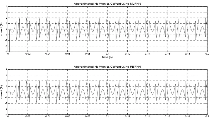
For harmonics current approximation, RBF neural network showed better performance than MLP. From the network complicity, MLP has more complicated network with two hidden layers while RBF consist only one hidden layer however RBF need more number of neuron compared with MLP. With same number of training data (200 data per cycles waveform), RBF has faster training process compared with MLP. SSE values stated that for function approximation purpose such as harmonics current waveform approximation, RBF showed better result than MLP. This result justified by lower SSE value for RBF than MLP. The approximated harmonics current component using RBF and MLP neural network for two kinds of non-linear loads were shown at Figures 6 and 7.
Figure 6 Approximated harmonics current using MLP and RBF for rectifier with resistive load
0 0.02 0.04 0.06 0.08 0.1 0.12 0.14 0.16 0.18 0.2
-1 -0.5 0 0.5 1
time (s)
c
ur
rent
(
A
)
Approximated Harmonics Current using MLPNN
0 0.02 0.04 0.06 0.08 0.1 0.12 0.14 0.16 0.18 0.2
-1 -0.5 0 0.5 1
time (s)
c
u
rre
n
t (A
)
Figure 7 Approximated harmonics current using MLP and RBF for rectifier with inductive load
0 0.02 0.04 0.06 0.08 0.1 0.12 0.14 0.16 0.18 0.2
-4 -3 -2 -1 0 1 2 3 4
time (s)
cur
ren
t (A
)
Approximated Harmonics Current using MLPNN
0 0.02 0.04 0.06 0.08 0.1 0.12 0.14 0.16 0.18 0.2
-4 -3 -2 -1 0 1 2 3 4
curren
t (A
)
Approximated Harmonics Current using RBFNN
The approximated harmonics current obtained from RBF and MLP used as reference signal for SAPF control. As mentioned before, the reference signal would be compared with carrier signal in PWM to generate switching signal. VSC-PWM would generate and inject compensation current to eliminate harmonics. The PWM should have a high switching frequency in order to reproduce accurately the compensating currents. In this research, 10 kHz switching frequency was used as PWM frequency. Interface low pass filter connected between VSC and the system to eliminate higher order harmonics around the switching frequency.
From simulation with constant load, THD value decreased from 25.6% became around 4% after the compensation with the proposed SAPF. The result showed that SAPF could improve performance of the system by eliminating harmonics current component from the source current. This indicated by small THD value and shape of source current became more sinusoidal. Source current waveform after and before compensated and compensation current from SAPF for various non-linear loads were shown at Figures 8 and 9.
Variable load simulation implemented to the system to verify whether MLP and RBF neural network still had ability to follow the load changing. For this simulation, two cases load changing would be analysed. Non-linear load modelled by uncontrolled rectifier which supplied 100 Ω resistive loads and changing twice in magnitude at 0.15 s and the other is 100 Ω and 0.1 H inductive load and changing by twice also at 0.15 s. After proposed SAPF installed to the system, source current improved.
Figure 8 Source current and compensation current for rectifier with resistive load, (a) based on MLPNN reference current (b) based on RBFNN reference current
0 0.02 0.04 0.06 0.08 0.1 0.12 0.14 0.16 0.18 0.2
-2 -1 0 1 2
time (s)
c
u
rre
n
t (A
)
Source Current before Compensated
0 0.02 0.04 0.06 0.08 0.1 0.12 0.14 0.16 0.18 0.2
-2 0 2
time (s)
c
u
rre
n
t (A
)
Compensation Current from SAPF based on MLPNN ref. Current
0 0.02 0.04 0.06 0.08 0.1 0.12 0.14 0.16 0.18 0.2
-2 -1 0 1 2
time (s)
c
u
rr
e
n
t (A
)
Source Current after Compensated
(a)
0 0.02 0.04 0.06 0.08 0.1 0.12 0.14 0.16 0.18 0.2
-2 -1 0 1 2
time (s)
c
u
rre
n
t (A
)
Source Current Before Compensated
0 0.02 0.04 0.06 0.08 0.1 0.12 0.14 0.16 0.18 0.2
-2 0 2
time (s)
c
u
rre
n
t (A
)
Compensation Current from SAPF based on RBFNN ref. Current
0 0.02 0.04 0.06 0.08 0.1 0.12 0.14 0.16 0.18 0.2
-2 -1 0 1 2
time (s)
c
u
rre
n
t (A
)
Source Current After Compensated
Figure 9 Source current and compensation current for rectifier with resistive load, (a) based on MLPNN reference current (b) based on RBFNN reference current
0 0.02 0.04 0.06 0.08 0.1 0.12 0.14 0.16 0.18 0.2 -5
0 5
time (s)
c
u
rr
ent
(
A
)
Source Current Before Compensated
0 0.02 0.04 0.06 0.08 0.1 0.12 0.14 0.16 0.18 0.2 -5
0 5
c
u
rre
n
t (A)
Compensation Current from SAPF based on MLPNN ref. Current
0 0.02 0.04 0.06 0.08 0.1 0.12 0.14 0.16 0.18 0.2 -5
0 5
time (s)
c
u
rre
n
t (A)
Source Current After Compensated
(a)
0 0.02 0.04 0.06 0.08 0.1 0.12 0.14 0.16 0.18 0.2 -5
0 5
time (s)
cu
rr
e
n
t (
A
)
Source Current Before Compensated
0 0.02 0.04 0.06 0.08 0.1 0.12 0.14 0.16 0.18 0.2 -5
0 5
time (s)
cu
rre
n
t (A
)
Compensation Current form SAPF based on RBFNN ref. Current
0 0.02 0.04 0.06 0.08 0.1 0.12 0.14 0.16 0.18 0.2 -5
0 5
time (s)
cu
rr
e
n
t (A
)
Source Current After Compensated
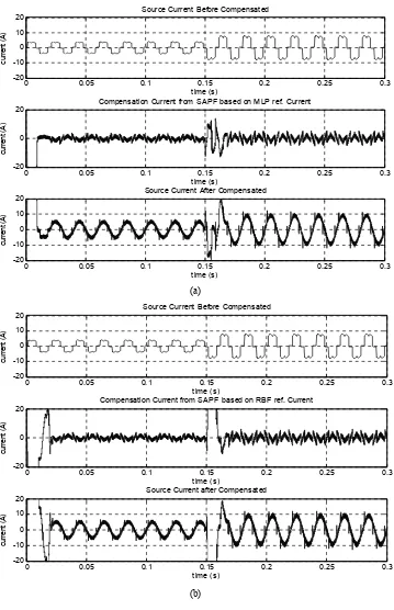
Figure 10 Source current and compensation current for rectifier with variable resistive load, (a) based on MLPNN reference current (b) based on RBFNN reference current
0 0.05 0.1 0.15 0.2 0.25 0.3
-20 -10 0 10 20
time (s)
c
u
rr
e
n
t (A)
Source Current Before Compensated
0 0.05 0.1 0.15 0.2 0.25 0.3
-20 0 20
time (s)
c
u
rr
e
n
t (A
)
Compensation Current from SAPF based on MLP ref. Current
0 0.05 0.1 0.15 0.2 0.25 0.3
-20 -10 0 10 20
time (s)
c
u
rr
e
n
t (A
)
Source Current After Compensated
(a)
0 0.05 0.1 0.15 0.2 0.25 0.3
-20 -10 0 10 20
time (s)
c
u
rr
e
n
t (A)
Source Current Before Compensated
0 0.05 0.1 0.15 0.2 0.25 0.3
-20 0 20
time (s)
c
u
rre
n
t (A
)
Compensation Current from SAPF based on RBF ref. Current
0 0.05 0.1 0.15 0.2 0.25 0.3
-20 -10 0 10 20
time (s)
c
u
rr
e
n
t (A)
Source Current after Compensated
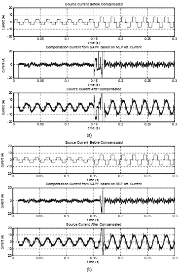
Figure 11 Source current and compensation current for rectifier with variable inductive load, (a) based on MLPNN reference current (b) based on RBFNN reference current
0 0.05 0.1 0.15 0.2 0.25 0.3
-20 -10 0 10 20
time (s)
c
u
rre
n
t (A
)
Source Current Before Compensated
0 0.05 0.1 0.15 0.2 0.25 0.3
-20 0 20
time (s)
cu
rr
e
n
t (
A
)
Compensation Current from SAPF based on MLP ref. Current
0 0.05 0.1 0.15 0.2 0.25 0.3
-20 -10 0 10 20
time (s)
cu
rr
e
n
t (
A
)
Source Current After Compensated
(a)
0 0.05 0.1 0.15 0.2 0.25 0.3
-20 -10 0 10 20
time (s)
c
ur
rent
(
A
)
Source Current Before Compensated
0 0.05 0.1 0.15 0.2 0.25 0.3
-20 0 20
time (s)
cu
rr
e
n
t (
A
)
Compensation Current from SAPF based on RBF ref. Current
0 0.05 0.1 0.15 0.2 0.25 0.3
-20 -10 0 10 20
time (s)
c
ur
rent
(
A
)
Source Current After Compensated
6 Conclusions
ANN could be implemented for signal approximation purpose well. RBF showed better performance than MLP for extracted and approximated harmonics current component from its original distorted current. RBF has smaller SSE, simpler architecture and faster training process. Unfortunately RBF has larger number of neuron than MLP but for overall the RBF showed superior performance than MLP.
The proposed method for SAPF control algorithm showed a good result. These methods could work properly not only for constant non-linear load but also for variable load changing in the system. THD value of source current decreased significantly from 25.6% for resistive load and 26.6% for inductive load become small between 3% to 5%. Source current also improved, indicated by more sinusoidal waveform which means almost all of harmonics current components have been eliminated.
References
Akagi, H., Watanabe, E.H. and Aredes, M. (2007) Instantaneous Power Theory and Application to
Power Conditioning, John Wiley & Sons, Inc., Hoboken, New Jersey.
Babaei. I. and Hosseini, S.H. (2010) ‘Development of modulation strategies for three-phase to two-phase matrix converters’, International Journal of Power Electronics, Vol. 2, No. 1, pp.81–106.
Chen, S. (2003) ‘Design of step dynamic voltage regulator for power quality enhancement’, IEEE
Trans. on Power Delivery, Vol. 18, No. 4, pp.1403–1409.
Chgangaroo, S., Srivastava, C., Thukaram, D. and Surapong, C. (1999) ‘Neural network based power system damping controller for SVC’, IEE Proceeding Part-C on Generation,
Transmission and Distribution, Vol. 146, No. 4, pp.370–376.
Hassoun, M.H. (1995) Fundamental of Artificial Neural Network, Asco Trade Typesetting Ltd., USA.
Mithulananthan, N. and Sode-Yome, A. (2004) ‘Comparison of shunt capacitor, SVC, and STATCOM in static voltage stability improvement’, IJEEE, Vol. 41, No. 2, pp.158–171. Shanthi, B. and Natarajan, S.P. (2010) ‘Comparative study on various unipolar PWM strategies for
single phase five-level cascaded inverter’, International Journal of Power Electronics, Vol. 2, No. 1, pp.36–50.
Tey, L.H. and So, P.L. (2002) ‘Neural network-controlled unified power quality conditioner for system harmonics compensation’, Proc. IEEE/PES Transmission and Distribution