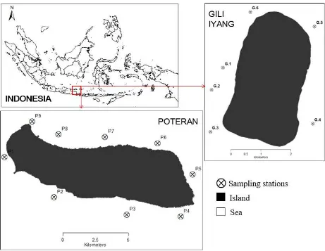
Estimation of TSS and Chl
-
a Concentration
from Landsat 8
-
OLI: The Effect of Atmosphere
and Retrieval Algorithm
Lalu Muhamad Jaelani1, Resti Limehuwey1, Nia Kurniadin1, Adjie Pamungkas2,
Eddy Setyo Koenhardono3, and Aries Sulisetyono4
AbstractTSS and Chl-a are globally known as a key parameter for regular seawater monitoring. Considering the high
temporal and spatial variations of water constituent, the remote sensing technique is an efficient and accurate method for extracting water physical parameters. The accuracy of estimated data derived from remote sensing depends on an accurate atmospheric correction algorithm and physical parameter retrieval algorithms. In this research, the accuracy of the atmospherically corrected product of USGS as well as the developed algorithms for estimating TSS and Chl-a concentration using Landsat 8-OLI data were evaluated. The data used in this study was collected from Poteran’s waters (9 stations) on April 22, 2015 and Gili Iyang’s waters (6 stations) on October 15, 2015. The low correlation between in situ and Landsat
Rrs(λ) (R2
= 0.106) indicated that atmospheric correction algorithm performed by USGS has a limitation. The TSS concentration retrieval algorithm produced an acceptable accuracy both over Poteran’s waters (RE of 4.60% and R2 of
0.628) and over Gili Iyang’s waters (RE of 14.82% and R2 of 0.345). Although the R2 lower than 0.5, the relative error was more accurate than the minimum requirement of 30%. Whereas, the Chl-a concentration retrieval algorithm produced an
acceptable result over Poteran’s waters (RE of 13.87% and R2 of 0.416) but failed over Gili Iyang’s waters (RE of 99.14%
and R2 of 0.090). The low correlation between measured and estimated TSS or Chl-a concentrations were caused not only by
the performance of developed TSS and Chl-a estimation retrieval algorithms but also the accuracy of atmospherically corrected reflectance of Landsat product.
Keywordsremote sensing; water quality; TSS; Chl-a.
AbstrakTSS dan Chl-a secara global dikenal sebagai parameter utama dalam pemantauan kualitas air laut. Mengingat
tingginya variasi temporal dan spasial dari konstituen perairan, teknik penginderaan jauh adalah metode yang efisien dan akurat untuk mengekstrak parameter fisik air tersebut. Akurasi dari parameter fisik yang diturunkan dari data penginderaan jauh tergantung pada algoritma koreksi atmosfer dan algoritma estimasi parameter fisik yang akurat. Dalam penelitian ini, akurasi dari produk USGS yang terkoreksi secara atmosfer serta algoritma yang dikembangkan untuk menghitung konsentrasi TSS dan Chl-a menggunakan Landsat 8-OLI data telah dikaji. Data yang digunakan dalam penelitian ini dikumpulkan dari Perairan Poteran (9 stasiun) pada tanggal 22 April 2015, dan Perairan Gili Iyang (6 stasiun) pada tanggal 15 Oktober 2015. Korelasi yang rendah antara data in situ dan Landsat Rrs(λ) (R2 = 0,106)
menunjukkan algoritma koreksi atmosfer yang digunakan oleh USGS memiliki keterbatasan. Algoritma estimasi konsentrasi TSS menghasilkan akurasi yang dapat diterima di Perairan Poteran (RE sebesar 4,60% dan R2 sebesar 0,628)
dan di perairan Gili Iyang (RE sebesar 14,82% dan R2 sebesar 0,345). Meskipun R2 lebih rendah dari 0,5, kesalahan relatifnya lebih akurat dari persyaratan minimum sebesar 30%. Sementara itu, algoritma estimasi konsentrasi Chl-a menghasilkan akurasi yang dapat diterima untuk Perairan Poteran (RE sebesar 13,87% dan R2 sebesar 0,416) akan tetapi
gagal di Perairan Gili Iyang (RE sebesar 99,14% dan R2 sebesar 0,090). Korelasi yang rendah antara konsentrai TSS atau
Chl-a estimasi dan ukuran disebabkan tidak hanya oleh akurasi algoritma estimasi TSS dan Chl-a, tetapi juga oleh akurasi dari reflektan terkoreksi atmosfer dari produk Landsat.
Kata Kuncipenginderaan jauh; kualitas air; TSS; Chl-a
I.INTRODUCTION1
emote sensing data have been widely used for monitoring the ecological, biological, and physical state of the seawater. Many studies have demonstrated that remote sensing imagery can be used for monitoring of the Chlorophyll-a (Chl-a) and Total Suspended Solid
1Lalu Muhamad Jaelani, Resti Limehuwey, and Nia Kurniadin,
Department of Geomatics Engineering, Faculty of Civil Engineering and Planning, Institut Teknologi Sepuluh Nopember, Surabaya, 60111, Indonesia. E-mail: [email protected], [email protected], [email protected].
2Adjie Pamungkas, Department of Urban and Regional Planning,
Faculty of Civil Engineering and Planning, Institut Teknologi Sepuluh Nopember, Surabaya, 60111, Indonesia. E-mail:[email protected].
3Eddy Setyo Koenhardono, Department of Marine Engineering,
Faculty of Marine Technology, Institut Teknologi Sepuluh Nopember, Surabaya, 60111, Indonesia. E-mail:[email protected].
4Aries Sulisetyono Department of Naval Architecture and
Shipbuilding Engineering, Faculty of Marine Technology, Institut Teknologi Sepuluh Nopember, Surabaya, 60111, Indonesia. E-mail: [email protected].
(TSS) concentrations. The range of 400 to 850 nm is often chosen for research aimed at determining methods for estimation of water quality parameters within the water column from remote sensing data [1]. The estimation of water quality parameters such as the concentration of TSS and Chl-a from satellite images is strongly depend on the accuracy of atmospheric correction and water quality parameter retrievals
algorithms [2]–[7]. Atmospheric correction is a
necessary process for quantitative monitoring of water quality parameters from satellite data.
In Indonesia’s water, there was very limited algorithm
developed and validated based on the in situ data of
physical parameter as well as its reflectance data [7], [8]. Hence, the existing algorithm that was designed in different water area was directly implemented without considering the dynamic changes and the specific characteristics of local water in Indonesia.
reflectance data processed by USGS, and 2) to develop more accurate TSS and Chl-a concentration retrieval algorithms for Landsat 8-OLI data at Poteran and Gili surrounding small islands in Indonesia. The first island is Poteran (7°5'11.88"S; 113°59'43.77"E), which is located in the southeast part of Madura Island, East Java
Province and has a surface area of 49.8 km2. At the south
of the island, local community utilizes sea for seaweed farming. The second one is Gili Iyang (6°59'7.07"S; 114°10'32.22"E) which is located in the northeast of Madura Island, East Java Province and has a surface area
of 9.15 km2. The concentration of oxygen in this island is
very high with average of 21.4 %. These two islands
To assess the performance of atmospheric corrected reflectance of Landsat product, the in situ spectra data and water quality concentration (i.e. TSS and Chl-a)
were collected from Poteran’s waters on April 22, 2015,
the same time with Landsat 8-OLI acquisition. The same
field campaign was performed over Gili Iyang’s waters
on October 15, 2015, except for spectra measurement which could not be measured by reason of strong wind speed. The data collecting station, which located less than one Landsat 8-OLI pixel (i.e. 30 m) away from the coastal area and corresponding Landsat 8-OLI pixels were contaminated by clouds were excluded from the analyses. Accordingly, 9 data (2 data without spectra) were used for Poteran area and 6 for Gili Iyang area.
All reflectance measurements were performed three hours before until three hours after 9.30 AM local time over optically deep waters. The water-leaving radiance
(Lu(λ)), the downward irradiance (Ed(λ)), and the
downward radiance of skylight (Lsky(λ)) were measured
at each site using a Field Spec Hand Held (or Pro VNIR) spectroradiometer (Analytical Spectral Devices, Boulder,
CO) in the range of 325–1075 nm at 1-nm intervals. The
above-water remote-sensing reflectance (Rrs(λ)) was
calculated approximately using the following equation [9]:
reference panel that has been accurately calibrated, and r
represents a weighted surface reflectance for the correction of surface-reflected skylight and is determined as a function of wind speed [9].
Concurrently, water samples were collected at nine and six stations over Poteran and Gili Iyang waters, respectively. Water samples were kept in ice boxes and taken to the laboratory for furthermore analysis. The chlorophyll-a were determined spectrometrically using
spectrophotometer. The optical density of the extracted
Chl-a was measured at four wavelengths (750, 663, 645,
and 630 nm), and the concentration was calculated
according to SCOR-UNESCO’s equations [10]. The total
suspended solids were determined gravimetrically. Samples were filtered through pre-combusted whatman gf/f filters at 500°c for 4 hours to remove dissolved organic matter in suspension, which was then dried at
105°c for 4 hours and weighted to obtain TSS. The in
situ remote sensing reflectance and water quality
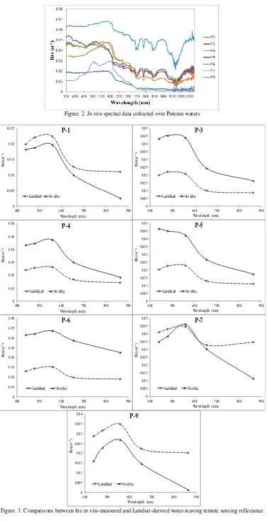
parameter collected over Poteran and Gili Iyang waters were presented in Table 1 and Figure 2.
Landsat 8-OLI Data Collection
Landsat 8-OLI data at path/row of 117/65 were collected at concurrent field campaign time. These data collected on April 22, 2015 and October 15, 2015. Since the atmospheric correction algorithm to convert remote sensing reflectance from Top of Atmospheric (TOA, recorded by sensor) to Bottom of Atmosphere (BOA, surface reflectance) is difficult for Landsat data, the Surface Reflectance (SR) which processed by USGS was used directly. The surface reflectance data was atmospheric corrected data using internal algorithm (for Landsat 8) and based on 6S algorithm for prior Landsat 8 for 7 bands. The information of Landsat band (excluded the TIR band) was presented in Table 2. These data
could be ordered and downloaded from ESPA’s website
(http://espa.cr.usgs.gov/). The downloaded SR data then calibrated by dividing all digital numbers by 10000 and
converted to remote sensing reflectance, Rrs(λ), by
dividing surface reflectance by π.
Accuracy Assessment
Assessment the accuracy of atmospheric correction algorithm developed by USGS and water quality parameter (TSS and Chl-a) retrieval algorithms used root
mean square error (RMSE), relative error (RE) and
The RMSE gives the absolute scattering of the retrieved
remote sensing reflectance as well as water quality
parameter concentration, the RE represents the
uncertainty associated with satellite-derived distribution and R2 the strong relationship between in situ measured
Rrs(λ) and estimated Rrs(λ) from atmospherically
corrected of Landsat 8-OLI as well as measured and estimated water quality parameter (TSS and Chl-a) concentrations.
III.RESULTS AND DISCUSSION
Validation of Landsat Remote Sensing Reflectance
To validate the atmospheric corrected reflectance of Landsat (SR), the average of 3-by-3 window of Landsat
pixel was used to compare with in situ-measured Rrs(λ)
potential error in spatial variability [11]. The in situ
remote sensing reflectance Rrs(λ) derived from Landsat
8 under estimate the in situ measurement Rrs(λ) at all
observation stations except at the observation station of 1, 7 and 9 where the data were overestimation. The low relationship between two set of data indicated by low determination coefficient (R2=0.106). However, all data
comparisons between in situ and Landsat derived remote
sensing reflectance have the same pattern.
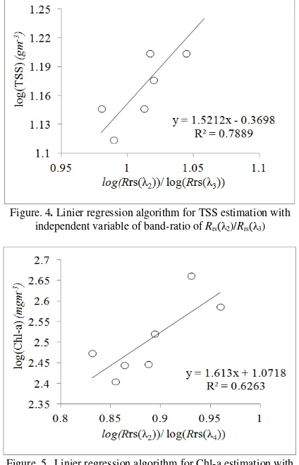
TSS Concentration Retrieval Algorithm
The total suspended sediment concentration retrieval algorithm developed using the regression algorithm
between the in situ TSS concentrations and in situ
measured remote sensing reflectance Rrs(λ) based on
single-band and two-band ratios reflectance
combinations. In situ TSS concentration and in situ
Rrs(λ) were used as dependent and independent variable,
respectively. From several combinations, the highest correlation between both variables indicated by the
highest coefficient of determination (R2) was chosen as a
retrieval algorithm. The regression algorithm for TSS concentrations was shown in Tables 3 and 4. In these The highest correlation produced by an algorithm based on Rrs(λ2)/Rrs(λ3) with R2 of 0.79. This band-ratio
based algorithm was used to calculate estimation of TSS concentration. The linier regression algorithm for TSS estimation with independent variable of band-ratio of
Rrs(λ2)/Rrs(λ3) was shown in Figure 4 and Equation 5.
Chl-a Concentration Retrieval Algorithm
The Chlorophyll-a concentration retrieval algorithm was made using regression algorithms based on single band and two band-ratios of Landsat 8 following the TSS retrieval algorithm. The regression algorithm of Chl-a concentrations were presented in Tables 5 and 6, for
single band and two band-ratio combinations,
respectively. In these tables, a high determination
coefficient (R2>0.5) were shown in band-ratio of
Rrs(λ1)/Rrs(λ4), Rrs(λ2)/Rrs(λ3), and Rrs(λ2)/Rrs(λ4) with
the highest correlation produced by Rrs(λ2)/Rrs(λ4) with
R2 of 0.63. The linier regression algorithm for Chl-a
estimation with independent variable of band-ratio of
Rrs(λ2)/Rrs(λ3) for Poteran’s waters was shown in Figure
5 and Equation 6.
log(𝐶ℎ𝑙 − 𝑎) = 1.613 (log 𝑅𝑟𝑠(𝜆2)
log 𝑅𝑟𝑠(𝜆4)) + 1.0718 (6) The algorithm produced the highest correlation with coefficient determination of 0.626.
Estimation of TSS Concentration and Its Validation
To assess the performance of the developed algorithms, the accuracy between measured data and estimated TSS
were tested using RMSE and RE. The comparisons
between the in situ-measured and Landsat-derived TSS
concentrations over Poteran and Gili Iyang’s waters were presented in Figures 5 and 6. Over Poteran’s waters, the
regression algorithm for estimating TSS concentration produced the highest accuracy with R2 of 0.628; RE of
4.60%; and RMSE of 1.124. Whereas, over Gili Iyang
waters, the algorithm produced the highest accuracy with
R2 of 0.345; RE of 14.823%; and RMSE of 2.916.
Estimation of Chl-a Concentration and Its Validation
The accuracy assessment of estimated Chl-a
concentration from Landsat data followed the same step as TSS assessment. The regression algorithm for
estimating Chl-a concentration over Poteran’s waters
produced high accuracy with R2 of 0.416; RE of
13.873%; and RMSE of 68.645. Whereas over Gili
Iyang’s waters, the R2, RE and RMSE were 0.090;
99.140% and 129.690, respectively (Figures 8 and 9). Spatial distribution of TSS and Chl-a concentrations were processed using the previous developed algorithms shown in Figure 10.
CONCLUSION
This study was performed over Poteran’s waters (9 stations) and Gili Iyang’s waters (6 stations). Over these
area, the in situ remote sensing reflectance Rrs(λ), Chl-a and TSS concentrations were collected as well as
Landsat-8 OLI data on the same acquisition time with in
situ data. Low correlation between in situ and Landsat
Rrs(λ) (R2=0.106) indicated that atmospheric correction
algorithm performed by USGS has a limitation. This phenomenon was also reported by Jaelani [12], using a
set of high quality in situ reflectance data collected over
Lake Kasumigaura, Japan.
The in situ data was used to develop an applicable physical parameter retrieval algorithm for Chl-a and TSS concentration. The accuracy of algorithms were assessed using in situ data collected at the same acquisition time of Landsat 8 satellite. The TSS concentration retrieval algorithm produced acceptable accuracy both over
Poteran’s waters (RE of 4.60% and R2 of 0.628) and over
Gili Iyang’s waters (RE of 14.82% and R2 of 0.345).
Although the R2 lower than 0.5, the RE was more
accurate than the minimum requirement of 30%. Whereas, the Chl-a concentration retrieval algorithm
produced acceptable result over Poteran (RE of 13.87%
and R2of 0.416) and failed over Gili Iyang’s waters (RE
of 99.14% and R2 of 0.090). This indicated that the accuracy of atmospheric corrected reflectances of Landsat product.
ACKNOWLEDGMENT
REFERENCES
[1] A. G. Dekker, "Detection of Optical Water Quality Parameters for Eutrophic Waters by High Resolution Remote Sensing," Vrije Universiteit, Amsterdam, 1993.
[2] K. G. Ruddick, F. Ovidio and M. Rijkeboer, "Atmospheric Correction of SeaWiFS Imagery for Turbid Coastal and Inland Waters," Applied Optics, vol. 39, no. 6, p. 897–912, 2000. [3] S. Sathyendranath, L. Prieur and A. Morel, "An Evaluation of The
Problems of Chlorophyll Retrieval from Ocean Colour, for Case 2 Waters," Advances in Space Research, vol. 7, no. 2, p. 27–30, 1987.
[4] W. Yang, B. Matsushita, J. Chen and T. Fukushima, "Estimating Constituent Concentrations in Case Ii Waters from MERIS Satellite Data by Semi-Analytical Model Optimizing and Look-Up Tables," Remote Sensing of Environment, vol. 115, no. 5, p. 1247–1259, 2011.
[5] L. M. Jaelani, B. Matsushita, W. Yang and T. Fukushima, "Evaluation of Four MERIS Atmospheric Correction Algorithms in Lake Kasumigaura, Japan," International Journal of Remote Sensing, vol. 34, no. 24, p. 8967–8985, 2013.
[6] L. M. Jaelani, B. Matsushita, W. Yang and T. Fukushima, "An Improved Atmospheric Correction Algorithm for Applying MERIS Data to Very Turbid Inland Waters," International Journal of Applied Earth Observation and Geoinformation, vol. 39, p. 128–141, 2015.
[7] N. Laili, F. Arafah, L. M. Jaelani, L. Subehi, A. Pamungkas, E. S. Koenhardono and A. Sulisetyono, "Development of Water Quality Parameter Retrieval Algorithms for Estimating Total Suspended Solids and chlorophyll-A Concentration using Landsat-8 Imagery," in Joint International Geoinformation Conference ISPRS Ann. Photogramm. Remote Sens. Spatial Inf. Sci., Kuala Lumpur, Malaysia, 2015.
[8] L. M. Jaelani, F. Setiawan and H. Wibowo, "Pemetaan Distribusi Spasial Konsentrasi Klorofil-A dengan Landsat 8 di Danau Matano dan Danau Towuti , Sulawesi Selatan," in Pertemuan Ilmiah Tahunan Masyarakat Ahli Penginderaan Jauh Indonesia XX, Bogor, 2015.
[9] C. D. Mobley, "Estimation of The Remote-Sensing Reflectance from Above-Surface Measurements," Applied Optics, vol. 38, no. 36, pp. 7442-7455, 1999.
[10] SCOR-UNESCO, "Determination of Photosynthetic Pigment in Seawater, Monographs on Oceanographic Methodology," UNESCO, Paris, 1966.
[11] L. Han and K. J. Jordan, "Estimating and Mapping Chlorophyll‐a Concentration in Pensacola Bay, Florida using Landsat ETM+ data," International Journal of Remote Sensing, vol. 26, no. 23, p. 5245–5254, 2005.
[12] L. M. Jaelani, F. Setiawan and B. Matsushita, "Uji Akurasi Produk Reflektan-Permukaan Landsat Menggunakan Data In situ di Danau Kasumigaura , Jepang," in Pertemuan Ilmiah Tahunan Masyarakat Ahli Penginderaan Jauh Indonesia XX, Bogor, 2015.
Figure. 2. In situ spectral data collected over Poteran waters
Figure. 3. Comparisons between the in situ-measured and Landsat-derived water-leaving remote sensing reflectance
0
400 500 600 700 800 900
Rrs
400 500 600 700 800 900
Rrs
400 500 600 700 800 900
Rrs
400 500 600 700 800 900
Rrs
400 500 600 700 800 900
Rrs
400 500 600 700 800 900
Rrs
400 500 600 700 800 900
Figure. 4. Linier regression algorithm for TSS estimation with independent variable of band-ratio of Rrs(λ2)/Rrs(λ3)
Figure. 5.Linier regression algorithm for Chl-a estimation with independent variable of band-ratio of Rrs(λ2)/Rrs(λ4)
Figure. 6. Comparisons between the in situ-measured and Landsat-derived TSS concentrations over Poteran’s waters
Figure. 7. Comparisons between the in situ-measured and Landsat-derived TSS concentrations over Gili Iyang’s waters
Figure. 8. Comparisons between the in situ-measured and Landsat-derived Chl-a concentrations over Poteran’s waters
Figure.9. Comparisons between the in situ-measured and Landsat-derived Chl-a concentration over Gili Iyang’s waters
TABLE 1.
IN SITU SPECTRAL AND WATER QUALITY
TABLE 2.
LANDSAT 8-OLI BAND INFORMATION
TABLE 3.
SINGLE BAND-BASED REGRESSION ALGORITHM FOR TSS WITH R2
Regresion Model Band 1 Band 2 Band 3 Band 4 Band 5
log(TSS)=y0 + a*bj 0.00 0.00 0.07 0.11 0.01
log(TSS)=y0 + a*log(bj) 0.00 0.00 0.06 0.10 0.00
TABLE 4.
TWO BAND RATIO-BASED REGRESSION ALGORITHM FOR TSS WITH R2
Regresion Model Band 1 Band 1 Band 1 Band 1 Band 2 Band 2 Band 3 Band 4 Band 5 Band 3 log(TSS)=y0 + a*(bj/bk) 0.17 0.43 0.77 0.01 0.72
log(TSS)=y0 + a*log(bj/bk) 0.15 0.39 0.77 0.00 0.72
log(TSS)=y0 + a*(log(bj)/log(bk)) 0.17 0.47 0.77 0.01 0.79
Model Regresi
Band 2 Band 2 Band 3 Band 3 Band 4
Band 4 Band 5 Band 4 Band 5 Band 5
log(TSS)=y0 + a*(bj/bk) 0.69 0.03 0.23 0.04 0.06
log(TSS)=y0 + a*log(bj/bk) 0.65 0.01 0.22 0.02 0.08
log(TSS)=y0 + a*(log(bj)/log(bk)) 0.73 0.00 0.24 0.04 0.14
TABLE 5.
SINGLE BAND-BASED REGRESSION ALGORITHM FOR CHL-A WITH R2
Regresion Model Band 1 Band 2 Band 3 Band 4 Band 5
log(chl-a)=y0 + a*bj 0.01 0.05 0.17 0.21 0.06
log(chl-a)=y0 + a*log(bj) 0.01 0.04 0.14 0.18 0.02
Station
Location Rrs (λ) (sr-1) TSS Chl Depth
Lat (°) Long (°) 440 nm 480 nm 560 nm 655 nm 865 nm (g/m3) (mg/m3) (m)
P-1 -7.0782 113.935 0.01823 0.01876 0.01971 0.01003 0.00255 14 278 3.8
P-2 -7.1058 113.969 0.0679 0.07301 0.06891 0.04308 0.04499 13 286 9
P-3 -7.1178 114.019 0.04327 0.04543 0.04396 0.02427 0.01624 13 298 10.1
P-4 -7.1191 114.056 0.0434 0.04474 0.04753 0.03017 0.01845 15 280 12.9
P-5 -7.0901 114.064 0.04661 0.04507 0.04237 0.02663 0.01729 14 254 8.5
P-6 -7.0686 114.04 0.06321 0.06442 0.06744 0.05746 0.0451 16 386 3.7
P-7 -7.0643 114.004 0.03498 0.03858 0.04618 0.03028 0.01151 18 459 4 P-8 -7.0624 113.972 0.10091 0.10964 0.11662 0.07857 0.07492 17 327 3.4
P-9 -7.0537 113.954 0.01594 0.02282 0.0268 0.01459 0.00122 16 332 13.9
Band Wavelength (nm) Central Wavelength Bandwidth (nm)
1 430 - 450 440 20
2 450 - 510 480 60
3 530 - 590 560 60
4 640 - 670 655 30
5 850 - 880 865 30
6 1570 - 1650 1610 80
TABLE 6.
TWO BAND RATIO-BASED REGRESSION ALGORITHM FOR CHL-A WITH R2
Regresion Model
Band 1 Band 1 Band 1 Band 1 Band 2
Band 2 Band 3 Band 4 Band 5 Band 3
log(chl-a)=y0 + a*(bj/bk) 0.10 0.00 0.61 0.00 0.50
log(chl-a)=y0 + a*log(bj/bk) 0.09 0.01 0.62 0.02 0.51
log(chl-a)=y0 + a*(log(bj)/log(bk)) 0.11 0.02 0.62 0.06 0.59
Model Regresi
Band 2 Band 2 Band 3 Band 3 Band 4
Band 4 Band 5 Band 4 Band 5 Band 5
log(chl-a)=y0 + a*(bj/bk) 0.57 0.00 0.24 0.00 0.01
log(chl-a)=y0 + a*log(bj/bk) 0.59 0.01 0.24 0.00 0.01