Estimating the Relative Free Energy of Different Molecular States with Respect to a Single
Reference State
Haiyan Liu, Alan E. Mark, and Wilfred F. van Gunsteren*
Laboratorium fu¨r Physikalische Chemie, Eidgeno¨ssische Technische Hochschule, ETH-Zentrum, CH 8092 Switzerland
ReceiVed: February 20, 1996X
We have investigated the feasibility of predicting free energy differences between a manifold of molecular states from a single simulation or ensemble representing one reference state. Two formulas that are based on the so-calledλ- coupling parameter approach are analyzed and compared: (i) expansion of the free energy
F(λ) into a Taylor series around a reference state (λ ) 0), and (ii) the so-called free energy perturbation formula. The results obtained by these extrapolation methods are compared to exact (target) values calculated by thermodynamic integration for mutations in two molecular systems: a model dipolar diatomic molecule in water, and a series of para-substituted phenols in water. For moderate charge redistribution (≈0.5 e), both extrapolation methods reproduce the exact free energy differences. For free energy changes due to a change of atom type or size, the Taylor expansion method fails completely, while the perturbation formula yields moderately accurate predictions. Both extrapolation methods fail when a mutation involves the creation or deletion of atoms, due to the poor sampling in the reference state simulation of the configurations that are important in the end states of interest. To overcome this sampling difficulty, a procedure based on the perturbation formula and on biasing the sampling in the reference state is proposed, in which soft-core interaction sites are incorporated into the Hamiltonian of the reference state at positions where atoms are to be created or deleted. For mutations going from p-methylphenol to the other five differently para-substituted phenols, the differences in free energy are correctly predicted using extrapolation based on a single simulation of a biased, non-physical reference state. Since a large number of mutations can be investigated using a recorded trajectory of a single simulation, the proposed method is potentially viable in practical applications such as drug design.
Introduction
In principle, the difference between the free energy of a reference state and another state of a system can be determined if the equilibrium fluctuations of the system in the reference state are completely known. Thus there exists the possibility of using extrapolation methods to predict the relative free energy of different states with respect to a given reference state from a single ensemble or simulation. In practice, when a computer-based molecular simulation technique such as Monte Carlo or molecular dynamics is used to generate the relevant ensemble,1-3 the region of configuration space that is sampled only corre-sponds to low-energy configurations of the state that is simulated. To obtain a meaningful estimate of the change in free energy associated with a given perturbation, the ensemble generated for the reference state must overlap with that for the alternative state. For this reason, simulations of intermediate states are generally used to ensure that sufficient overlap is achieved within a finite simulation time. When using interme-diate states, each different mutation of the system requires a different pathway composed of intermediate states. Separate simulations must be carried out at a number of different intermediate states along different pathways, each of which is computationally expensive. Thus, although free energy calcula-tions have been shown to give accurate results under certain circumstances,4,5substantial computational cost is often associ-ated with obtaining a single number. This fact greatly inhibits wider application of this methodology. For example, free energy calculations are unsuitable for screening a large number of
compounds or for guiding experimental planning in drug design. For such purposes, methods that rapidly predict changes in the binding constant of a ligand associated with specific modifica-tions are highly sought after.
There have been several previous studies aimed at the prediction of the change in free energy associated with multiple perturbed states from a single simulation. In earlier work by this group,6 the first-order derivatives of the change in free energy associated with modifications at different atomic sites were computed from a single simulation of the reference state. A linear combination of these first-order derivatives was then used to approximate the total change in free energy associated with a certain alternative state. The relative binding constants of different trimethoprim analogues with dihydrofolate reductase were estimated using this approach. Unfortunately, the results showed little correlation with experimental data, suggesting that the approximation was too crude. In later work of Smith et
al.,7the free energy as a function of the coupling parameterλ was expanded into a Taylor series around λ ) 0, which corresponds to the reference state. Using a 1 ns simulation, the authors showed that for predicting the free energy changes associated with substantial charge rearrangements of a model diatomic dipolar molecule in water, truncating the series beyond the second- or third-order terms gave results in good agreement with thermodynamic-integration calculations. Higher-order derivatives, however, converged slowly. Similar approaches described earlier by Levy et al.8and King and Barford9can be shown to be equivalent to including only the first- and the second-order terms in the Taylor series.7 The approach of King and Barford, based on the linear response theory, gave accurate estimates for the change in free energy associated with creating * To whom correspondence should be addressed.
XAbstract published in AdVance ACS Abstracts, May 1, 1996.
a net charge in solution. The method is, however, dependent on a simulation of a mixed state which is a linear combination of the two end states. The approach of Smith et al.7does not involve such restrictions and considering the significant charge rearrangements involved in the dipolar diatomic solute ((0.25
e),7 the results were encouraging in regard to the predictive power of extrapolation approaches. However, several problems remained to be solved.
First, if the infinite Taylor series converges, it is formally equivalent to the free energy perturbation formula using a single window. This raises the question of whether extrapolation based on the perturbation formula is more general and more efficient than that based on the Taylor series expansion. Second, although extrapolation based on a series expansion worked well for charge rearrangements, it is not clear whether it is appropriate for other types of chemical modifications, such as changes in van der Waals parameters, and the creation or deletion of atoms. Here, we show that the perturbation formula can in fact be used to accurately predict the changes in free energy associated with charge rearrangement and modest changes in van der Waals parameters for a range of chemically relevant mutations from a single simulation of a reference state. The method may fail, however, for mutations involving the creation or deletion of atoms. In these cases, configurations corresponding to low-energy parts of the configuration space for the perturbed state cannot be sampled during a simulation of the reference state. We demonstrate, however, that this difficulty can be overcome by the incorporation of a general biasing potential energy term into the Hamiltonian of the reference state. At positions where atoms are to be created or deleted, soft interaction sites are introduced which interact with the surroundings via a modified Lennard-Jones 6-12 interaction which approaches a finite value at short interatomic distances. The introduction of such interaction sites extends the parts of configuration space that can be sampled in the reference state such that it encompasses the parts of configuration space accessible to the system in relevant alternative states. The free energy changes associated with changing the system from the nonphysical reference state to the physical alternative states are then calculated by applying the perturbation formula.
In this work two systems are analyzed. The first system is a model dipolar diatomic molecule in water (dipole/water system), identical to that used by Smith et al.7 The second system consists of a series of para-substituted phenols in water (phenol/water system), which has previously been the subject of extensive thermodynamic studies.10 Theoretical aspects of the calculations are summarized in the next section. Details of the computations are then given. To test the methodology, results from application of the perturbation formula are com-pared with those from thermodynamic-integration calculations and those obtained using a truncated Taylor series. The energetic and entropic contributions to the total free energy change associated with changing the dipole moment of a simple diatomic molecule in water are also discussed.
Theory
Consider the free energy difference between two systems, A and B, described by the Hamiltonians HAand HB, respectively. An intermediate state with the Hamiltonian H(λ) can be constructed such that H(0) )HAand H(1) )HB, whereλis the coupling parameter. For example, in the case of linear coupling
As the Hamiltonian, H(λ), is a function ofλ, the free energy of the system, F, will also be a function ofλ, F(λ). It can be shown that the first derivative of F(λ) is11
where 〈...〉λ denotes an average over the ensemble at the correspondingλvalue. The difference in free energy between the states B and A is given by11
Formulas 2 and 3 are the theoretical foundation of the so-called thermodynamic-integration method.11
Formally, F(λ) can also be expanded into a Taylor series at λ)0,7
where the values of the higher-order derivatives F′′, F′′′, ... at λ)0 can be computed as averages over the ensemble of the reference state.7 For example, assuming linear coupling of the Hamiltonian withλ, the second-order derivative is7
where kBis the Boltzmann constant and T is the temperature. It is important to emphasize that the expansion in formula 4 is only valid forλvalues within the radius of convergence of the Taylor series.
An alternative to thermodynamic integration is to compute the difference in free energy between two states of a system directly using the free energy perturbation formula.12 It can be shown that
Extrapolation methods to estimate changes in free energy from a single simulation can either be based on the series expansion formula 4 or on the perturbation formula 6. The two formulas are equivalent as long as the Taylor series converges. However, the two expressions are no longer equivalent if the series is truncated at a certain term in formula 4. This is always necessary in practice. By truncating the series it is assumed that the free energy is a smooth function ofλand that higher order derivatives, which converge slowly, are zero. The derivatives of various order are dependent on theλ-coupling scheme, that is, the chosen functional form of H(λ). Thus, the convergence of the series or the point at which the assumption inherent in the truncation becomes valid will depend on the coupling scheme used. Truncation of the series implicitly smooths the free energy curve. In certain cases, truncating the Taylor series will lead to better converged estimates of the change in free energy by neglecting irrelevant but noisy higher order terms. In contrast, using the perturbation formula all higher order terms are implicitly included.
Using the perturbation formula the ensemble of the alternate state is extrapolated from the ensemble of the reference state. The reliability of the results thus obtained is highly dependent on whether the configurations sampled at the reference state are representative of the ensemble as a whole. A well-known problem in free energy calculations is that low-energy regions of the configurational space in the reference state do not correspond to low-energy regions in the end state when atoms
are created or deleted.13-16 Thus it is to be expected that for mutations involving the creation or deletion of atoms, the relevant parts of configuration space of the system at different perturbed states will not be accessible to the system, and reliable predictions of free energy changes cannot be made based on a single simulation. However, this is only true if the reference state directly corresponds to a specific physical state. In principle, the difference in free energy for any perturbed state of interest can be estimated as long as the reference state is defined such that the parts of configuration space sampled by the system encompasses those parts which are relevant to all physical states of interest. This can be achieved by incorporat-ing an appropriate biasincorporat-ing or umbrella potential energy term into the Hamiltonian of a given physical reference state. For the creation or deletion of atoms, a so-called soft-core interaction function can serve as an appropriate umbrella potential energy term. A recently proposed soft-core interaction function has the form16
whereǫijandσijhave their normal meanings as in a
Lennard-Jones function. The distance between atoms i and j is denoted by rij. The parameter R determines the “softness” of the
interaction. The interaction is referred as soft, as unlike the normal Lennard-Jones interaction, the interaction energy in formula 7 approaches a finite value as rij approaches zero.
Placing soft-core interaction sites with an appropriateRvalue at locations where atoms are to be created or deleted acts to penalize configurations without any cavity at those sites, while still permitting solvent molecules to occasionally occupy these locations. The free energy difference between a physical state and the nonphysical reference state can be calculated using the perturbation formula 6, and the free energy difference between the different physical states themselves can then be calculated by constructing thermodynamic cycles.
Computational Details
Dipole/Water System. The dipole/water system used is the
same as that used by Smith et al.7 The system consists of a dipolar diatomic molecule in a box containing 510 SPC/E17 water molecules. The two atoms of the molecule have the same Lennard-Jones interaction parameters as the oxygen atoms of the surrounding water molecules and bear opposite charges ((0.25 e). They are separated by a rigid bond of length 0.2 nm. Parameters used in the simulation were the same as described by Smith et al.7 Two perturbed states were consid-ered. In the first perturbed state corresponding toλ )1, the sign of the charge on each of the two atoms is inverted. For this mutation, the change in free energy∆F(1) is zero as the
reference and the perturbed states are equivalent. In the second perturbed state,λ) -1, the charges on each atom are increased to(0.75 e. Thus the statesλ)1, 0.5,-0.5, and-1 correspond to inverting, eliminating, doubling, and tripling the dipole moment, respectively.
A 500 ps simulation of the reference state (λ ) 0) was performed during which the molecular configurations were recorded every 0.004 ps. The change in free energy for values ofλ between-1 and 1 was then calculated using formula 6. The energetic contribution ∆U and the entropic contribution T∆S to the total free energy change were also calculated as
functions of λusing
and
where∆V(λ) stands for V(λ)-V(0).
Phenol/Water System. The second system considered involves mutations between a series of para-substituted phenol molecules in water. Three different reference states were investigated. The first reference state consists of one p-methylphenol molecule in a truncated-octahedron box containing 544 SPC18water molecules. The setup for the simulation was the same as that used by Mark et al.10 The potential energy function parameters for p-methylphenol are listed in Table 1. Also listed in Table 1 are the parameters for p-chlorophenol,
p-cyanophenol, and p-methoxyphenol, which served as
alterna-tive perturbed or end states to which the change in free energy was estimated. A 300 ps simulation of p-methylphenol in water was carried out during which the Cartesian coordinates of all atoms were recorded every 0.004 ps at a precision of 10-8nm. The estimation of the change in free energy from this reference state to each perturbed state was carried out using the recorded set of configurations. For this estimation, only interactions involving perturbed atoms need to be determined for each configuration. Thus this approach is computationally much more efficient than repeating the entire simulation for each different mutation. In the free energy estimation step, the atomic coordinates of a new substitution group were generated for each time frame using standard geometries for the chemical moieties, while interactions involving the old substitution group were switched off. Three alternative physical perturbed states were considered in which the-CH3group was perturbed into either a-Cl group, a-CN group, or a-OCH3group. The change in free energy to each end state was calculated using the Taylor series truncated beyond the fourth-order derivative and using the perturbation formula (formula 6).
To examine in more detail the process of the creation and deletion of atoms, two additional perturbed states not considered by Mark et al.10were also investigated. In the first the-CH
3 group of p-methylphenol was mutated to a dummy atom. In the second the-CH3group was not changed but an additional -CH3group was created at the position corresponding to that of the methyl group in p-methoxyphenol. In addition to calculating the change in free energy associated with the mutation from p-methylphenol to each of these two perturbed states using both formula 4 and formula 6, these two end states were used to investigate the effect of using nonlinear coupling schemes for the Lennard-Jones interaction on the accuracy of predictions based on a series expansion. The linear coupling scheme was compared with a soft-core coupling scheme in which the Lennard-Jones interaction between atom pairs had the form
Hamiltonian. However, the first-order derivatives will be zero atλ)0 using these schemes. This makes them less suitable for use in extrapolation procedures based on a Taylor series expansion, as the results are determined by higher-order derivatives which converge slowly.
Simulations of two nonphysical reference states were also carried out. In the first, which will be referred to as Sa, three soft interaction sites, one replacing the -CH3 group of the p-methoxyphenol, the other two corresponding to the oxygen
atom of p-methoxyphenol and the -CH3 group of p-methyl-phenol, were used. In the second nonphysical reference state,
which will be referred to as Sb, again three soft interaction sites were included, the first, as in Sa, replacing the-CH3group of p-methoxyphenol, the second and the third placed at positions
corresponding to the nitrogen atom of p-cyanophenol and the chloride atom of p-chlorophenol, respectively. TheRparameter in formula 7 was set to 0.6. There was no charge on the soft atoms. The bonded interactions were taken equal to those of the corresponding physical states. Where necessary, dummy atoms with only bonded interactions were added to link the soft atoms to the phenol ring. The change in free energy associated with going from each of these two nonphysical reference states to each of the five perturbed states of interest mentioned above as well as to the p-methylphenol reference state were estimated by applying the perturbation formula (formula 6) to a 300 ps simulation of the appropriate reference state. The same method was used to estimate the difference in free energy between Sa and Sb. For comparison, the 300 ps simulation of p-methyl-phenol in water was also used to estimate the change in free energy going from p-methylphenol to both Saand Sb.
To obtain reference or target values for the change in free energy against which extrapolation values using a single simulation could be compared, full thermodynamic integration calculations were also performed for the mutations of p-methylphenol into p-chlorophenol, p-cyanophenol, p-methoxy-phenol, and the two states used to investigate the effect of the creation or deletion of atoms. Simulations were performed at 10-15λvalues between 0 and 1. Linear coupling was used. At eachλvalue, F′(λ) was computed according to formula 2 using 5 ps equilibration followed by 50 ps sampling. ∆F(λ) was obtained by numerical integration using the trapezoidal method. In the calculations presented here, contributions to the change in free energy arising from changes in bonded interaction terms have, for simplicity, not been included. For this reason the calculated values from Mark et al.10cannot be compared directly to the extrapolation and thermodynamic integration values presented here. For an approximate method, this simplification is justified as these contributions can largely cancel within a thermodynamic cycle.
Results and Discussion
Dipole/Water System. The change in free energy associated
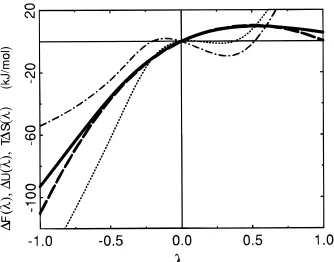
with increasing or inverting the dipole moment of the diatomic solute of the dipole/water system as a function ofλis shown in Figure 1. The numerical results are listed in Table 2. The TABLE 1: Force Field Parameters Used for
Para-Substituted Phenols10 a
phenol H1 0.398 0.0 0
O1 -0.548 23.25 421/600
C1 0.15 23.65 898
p-CN N -0.368 24.13 636/900
C 0.184 23.65 898
aThe interaction function is described in ref 19.bLennard-Jones
parameters C6(i,j) and C12(i,j) were obtained using the following
combination rules: C6(i,j))[C6(i,i)]1/2* [C6(j,j)]1/2and C12(i,j))[C
12(i,i)]1/2[C12(j,j)]1/2. The Lennard-Jones parameters for Cl atom
cor-respond to values for the Cl-anion in the GROMOS force field,19which
lead to larger van der Waals radius for the Cl atom than the parameters
used by Mark et al.10 cTo mimic the effects of hydrogen bonds, the
C12parameters of polar atoms were increased for hydrogen bond donor
and acceptor pairs. This is the second value in this column.dThe
charge on the C4 atom was opposite that of the para-substituent so that a neutral group was obtained.
Figure 1. Extrapolation (formula 6, solid line) and target
thermody-namic integration (dashed line) change in free energy∆F(λ))F(λ)
-F(0) as a function ofλfor the dipole/water system. The extrapolation
energetic (∆U(λ), formula 8, dotted line) and entropic (T∆S(λ), formula
9, dot-dashed line) contributions are also shown. Extrapolation values are obtained by applying the perturbation formula 6 to a 500 ps
simulation atλ)0. The target data is obtained by thermodynamic
integration using the first-order derivatives calculated from simulations
dashed line in Figure 1 corresponds to the target thermodynamic-integration values. This curve was computed using the deriva-tives taken from Smith et al.7obtained by performing simula-tions at nine differentλvalues. In Table 2, the extrapolation values from Smith et al., which were calculated using the truncated (beyond the first to beyond the fifth order) Taylor series,7have also been included. Extrapolation based on a single 1000 ps simulation using the truncated (beyond the third order) Taylor series and extrapolation based on a single 500 ps simulation using the perturbation formula are both able to reproduce the change in free energy obtained from thermody-namic integration in the rangeλ) -0.5 toλ)0.5. Outside this range, extrapolation based on applying the perturbation formula yields a too large free energy difference while that based on the truncated Taylor series gives oscillating results upon including derivatives of increasingly higher order (Table 2).
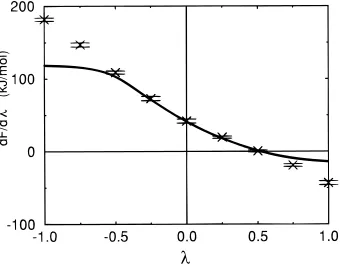
The first-order derivative of ∆F(λ) with respect toλ was obtained as a function ofλby taking the numerical derivative of the curve ∆F(λ) generated by applying the perturbation formula. The resulting curve is shown in Figure 2 together with the target derivatives directly calculated from simulations at differentλvalues.7 Forλvalues outside the range-0.5 to 0.5, the extrapolation value of the first-order derivative deviates from
the target values and approaches a constant value. The extrapolation second-order derivative approaches zero. Smith
et al.7pointed out that the second-order derivative represents the change of the ensemble with λ. One way to interpret formula 6 is to consider the ensemble at differentλvalues as being extrapolated from the ensemble sampled atλ)0. The ensemble at a givenλvalue is obtained by changing the relative weight of each configuration sampled atλ)0 in proportion to exp{-[V(λ) - V(0)]/kBT}. When the deviation from the reference state is large, the extrapolated ensemble will be dominated by a small number of configurations for which the weights are significant. As the dominating configurations do change little withλ, the extrapolation second-order derivative approaches zero.
Because the extrapolated ensemble becomes dominated by a small fraction of the configurations sampled, the extrapolation change in free energy is subject to serious statistical uncertainty when the deviation from the reference state is large. This is demonstrated in Figure 3, which shows the convergence of the extrapolation change in free energy as a function of the length of the simulation. The values are obtained using the perturbation formula 6. The most significant feature of these plots is the sudden decrease of the extrapolation values at various time points. These points correspond to times at which a new configuration is sampled, for which the VB-VAvalue is much smaller than those previously sampled. Once sampled, the new configuration dominates the ensemble average. Because VB -VAis proportional to the deviation ofλfrom zero, the sudden drops are magnified as the deviation increases. For comparison, the convergence of the change in free energy for λ ) -1 extrapolated using a Taylor series truncated beyond the second order is also included in Figure 3. Because the first-order derivative of the free energy with respect toλis the average of
VB - VA (formula 2) and the second-order derivative is proportional to the fluctuation of VB - VA (formula 5), the ensemble averages of these terms converge much faster than the change in free energy based on application of the perturba-tion formula. However, the ensemble averages of higher-order derivatives converge extremely slowly.7 As the deviation from the reference state increases, the Taylor series itself also converges more slowly. This is evident from the oscillation of the extrapolated values upon the inclusion of higher-order derivatives in the series (Table 2).
From the 500 ps simulation atλ)0, the extrapolation change in free energy as a function ofλwas partitioned into an internal energy contribution and an entropy contribution. The results are included in Figure 1. It is well-known that it is more difficult to obtain accurate relative entropies and internal energies than TABLE 2: Free Energy Changes (in kJ mol-1) Associated
with the Process of Charge Rearrangement of a Model Dipolar Diatomic Molecule in Water
λa -1.0 -0.5 0 0.5 1.0
target valuesb
thermodynamic integration7 -109.97 -36.78 0 9.97 0.09
extrapolation valuesc
Taylor expansion of order7
1 -41.63 -20.82 0 20.82 41.63
2 -97.44 -34.77 0 6.87 -14.17
3 -119.54 -37.53 0 9.63 7.93
4 -117.35 -37.40 0 9.77 10.12
5 -101.32 -36.90 0 9.27 -5.91
perturbation formula
-93.0 -35.9 0 9.5 5.4
aCharges on the two solute atoms were(0.75 e (λ) -1.0),(0.5
e (λ) -0.5),(0.25 e (λ)0), 0 (λ)0.5), and-0.25 e (λ)1.0),
respectively.bTaken from Smith et al.7 They were obtained by
thermodynamic integration using the first-order derivatives calculated
from simulations at nine different λ values and using numerical
integration.cIn the rows labeled 1-5 the extrapolation results obtained
using the Taylor series truncated beyond terms of the corresponding
order (taken from Smith et al.7) are listed. The derivatives were
computed from a 1 ns simulation at the reference stateλ)0. In the
last row the extrapolation results obtained by directly applying the
perturbation formula to a 500 ps simulation at the reference stateλ)
0 are listed.
Figure 2. Extrapolation (solid line) and target (crosses) first-order
derivatives of the free energy with respect to λfor the dipole/water
system. The extrapolation data are obtained by numerical differentiation
of the extrapolation∆F (λ) (formula 6). The target data is taken from
Smith et al.7
Figure 3. Convergence of the extrapolated change in free energy for
the dipole/water system. The values are obtained using the perturbation
formula 6 (solid lines). Forλ) -1, convergence of the extrapolation
to obtain accurate relative free energies. To estimate the relative magnitude of the errors involved in the extrapolations, the 500 ps trajectory was partitioned into five 100 ps trajectories, and the standard deviation for each of the averaged quantities was calculated. The results are shown in Figure 4. At differentλ values, the standard deviations of the extrapolation internal energy and entropic contributions are always an order of magnitude larger than that of the extrapolation overall change in free energy. Nevertheless, the shape of the extrapolation T∆S
curve in Figure 1 is of particular interest. The curve is expected to be symmetric by inversion about the lineλ)0.5. Clearly, the values for larger changes inλare not reliable. However, at λ)0.25, the extrapolation T∆S value is ca.-9 kJ mol-1and the standard deviation is ca. 3 kJ mol-1. Starting from the point λ)0 and increasingλ, the entropy of the system will initially decrease, while the change in internal energy will be relatively small. Physically this process corresponds to a reduction of the dipole moment of the diatomic solute. This decrease in entropy is consistent with the belief that the hydration of a nonpolar solute is entropically unfavoured. For λ going to negative values, the polarity of the solute is increased further, and the entropy of the system passes through a maximum before it decreases again. The overall change in free energy remains negative, resulting from the negative change in internal energy which then dominates.
Phenol/Water System with Physical Reference State. The
differences in free energy associated with changing p-meth-ylphenol to p-chlorophenol, p-cyanophenol, and p-methoxy-phenol in water were extrapolated using the 300 ps simulation of p-methylphenol in water and are listed in Table 3, together with values obtained from full thermodynamic-integration calculations.
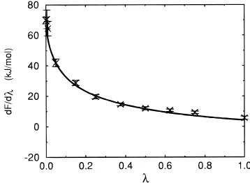
For the two cases in which the end states do not involve the creation of a bulky methyl group (chlorophenol and p-cyanophenol), the values obtained by applying the perturbation formula to the p-methylphenol ensemble and the results obtained by thermodynamic-integration calculations agree within 2.5 kJ mol-1. Figure 5 shows the extrapolation values of the first-order derivative of∆F(λ) along with values determined from simulations at different λvalues for the p-chlorophenol case. The agreement within the entire λrange from 0 to 1 suggests that the configurations sampled during the 300 ps simulation of p-methylphenol (λ)0) can effectively be used to represent an ensemble appropriate for p-chlorophenol (λ)1) or for any intermediateλvalue.
When the methyl group is changed into a methoxy group the extrapolation change in free energy deviates from the value obtained by thermodynamic integration by 18.4 kJ mol-1(Table 3). This is due to the fact that a new methyl group is to be
created at a position where no cavity exists in any of the sampled configurations. The same effect is observed when a methyl group is added to p-methylphenol. The extrapolation change in free energy deviates from the target thermodynamic-integra-tion value by 16.7 kJ mol-1(Table 4). Conversely, when the methyl group of p-methylphenol is deleted, the sampled configurations always contain a cavity at the methyl group position and thus cannot be used to represent the ensemble of the end state. Consequently, the extrapolation change in free energy deviates from the expected value by 7.1 kJ mol-1(Table 4). The extrapolation change in free energy associated with the deletion of the methyl group as a function ofλis shown in Figure 6, together with the change in free energy calculated using thermodynamic integration. Significant deviation between the extrapolation and the thermodynamic-integration values occurs only asλapproaches 1. This is a consequence of the
Figure 4. Standard deviations over five values of the extrapolation
change in free energy (solid line), energetic (dashed line), and entropic (dotted line) contributions for the water/dipole system, calculated by partitioning the simulation into five 100 ps blocks.
TABLE 3: Free Energy Changes (in kJ mol-1) Associated with Modifications of the-CH3Group of p-Methylphenol in Water
mutation CH3to Cl
CH3
to CN
CH3
to OCH3
target valuesa
thermodynamic integration 17.1 -9.5 8.0
extrapolation valuesb
Taylor expansion of order
1 69.9 104.8 973.0
2 -1.1×10³ -1.6×10⁴ -5.9×10⁶
3 1.1×10⁵ 1.7×10⁷ 1.9×10¹¹
4 -1.7×10⁷ -2.1×10¹⁰ -6.9×10¹⁵
perturbation formula reference state
-CH3: R )0.0 15.8 -7.2 26.4
-Sa: R )0.6 17.7 -5.1 4.7
-Sb:R )0.6 17.4 -6.0 7.5
aThe target values were obtained by thermodynamic integration
using simulations at 10 to 15 different λ values and numerical
integration.bIn the rows labeled 1-4 the extrapolation results obtained
using Taylor series (expanded aroundλ)0) truncated beyond terms
of the corresponding order are listed. The derivatives were calculated from a 300 ps simulation of the reference state p-methylphenol in water. In the bottom three rows extrapolation results obtained by applying the perturbation formula to 300 ps simulations of three different reference states are listed. The extrapolation results obtained by applying the perturbation formula and thermodynamic cycles using the
300 ps simulations of the non-physical reference states Saand Sbin
which the van der Waals interactions between certain atoms were
computed using (7) withR )0.6 as described in the text are indicated
by Saand Sb, respectively.
Figure 5. Extrapolation (solid line) and target (crosses) first-order
derivatives of the change in free energy associated with changing p-methylphenol into p-chlorophenol in water. The extrapolation data is obtained by using a 300 ps simulation of p-methylphenol in water, applying the perturbation formula 6 and numerically differentiating the
resulting∆F(λ). The target data is computed from 50 ps simulations
at the correspondingλvalues. The error bars for the target data are
linear coupling scheme in formula 10 for R ) 0, in which significant shrinking of the effective van der Waals radius of the methyl group takes place only whenλ is very close to 1. The contribution from the cavity term to the total change in free energy is, however, about 7 kJ mol-1in this case and cannot be neglected.
In all cases investigated using the phenol/water system, the Taylor series with linear coupling does not converge (Tables 3 and 4). Thus extrapolations based on the series expansion are unreliable. In principle, the convergence properties of the Taylor series can be affected by changing the λ dependence of the Hamiltonian. Therefore, the reliability of extrapolations based on a truncated Taylor series is potentially dependent on the coupling scheme. In Table 4 we include the extrapolation values based on the Taylor series truncated beyond the second order and with a soft-core interaction in theλ-dependent Hamiltonian,
e.g., formula 10. Two differentR-parameter values were used in the soft-core interaction. The extrapolation change in free energy is highly dependent on the value of the parameter R and thus hardly useful.
For processes that involve only charge rearrangement, the range over which both extrapolation methods are valid is quite
encouraging.7 In practice, extrapolation based on the application of the perturbation formula is the easier to implement. It is also more general in that it can deal with small changes in the van der Waals radius (or excluded volume) of a solute, cases where extrapolation based on the truncated series clearly fails when using linear coupling. However, using the perturbation formula, it is not possible to accurately calculate the change in free energy associated with the creation or elimination of atoms based on a single simulation of a physically meaningful reference state.
Phenol/Water System with Nonphysical Reference State.
The change in free energy associated with the mutation of the phenol/water system from each of the two nonphysical reference states to different physical end states was calculated by applying the perturbation formula. The end states investigated include
p-methylphenol, p-chlorophenol, p-cyanophenol, and the two
states involving addition or deletion of a methyl group to or from p-methylphenol, respectively. The results are listed in Table 5. In order to compare the results directly to the values obtained using p-methylphenol as a reference state, the changes in free energy have been converted to free energies relative to
p-methylphenol by constructing thermodynamic cycles. The
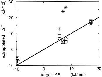
results are included in Tables 3 and 4. Figure 7 illustrates the degree of agreement between the change in free energy calculated using thermodynamic integration and that extrapolated using the perturbation formula and simulations of only the TABLE 4: Free Energy Changes (in kJ mol-1) Associated
with Changing the Methyl Group of p-Methylphenol into a Dummy Atom and Adding a Methyl Group to
p-Methylphenol
modification CH3to dummy CH3to CH3+CH3
target valuesa
thermodynamic integration 5.7 7.1
extrapolation valuesb
Taylor expansion truncated beyond the second order
hard core: R )0.0 15.5 -4.0×10⁴
soft core: R )0.1 14.5 -1209.4
soft core: R )0.5 10.6 20.6
perturbation formula reference state
-CH3: R )0.0 12.8 23.8
-Sa: R )0.6 8.3 5.4
-Sb: R )0.6 6.4 4.6
aThe target values were obtained by thermodynamic integration
using simulations at 13 differentλvalues and numerical integration.
bThe next three rows list extrapolation values based on the Taylor series
truncated beyond the second order. Different coupling schemes
between the Hamiltonian and λwere used (eq 10): hard core (R )
0.0) and soft core (R )0.1 andR )0.5); the extrapolation results of
applying the perturbation formula were obtained as described in the footnote of Table 3.
Figure 6. Extrapolation (solid line) and target (dashed line) change
in free energy as a function ofλassociated with the deletion of the
methyl group of p-methylphenol. The extrapolation data is obtained by using a 300 ps simulation of p-methylphenol in water and applying the perturbation formula 6. The target data is obtained by
thermody-namic integration calculation using simulation at 13 differentλvalues
and numerical integration.
TABLE 5: Free Energy Differences (in kJ mol-1) between the Nonphysical Reference States with Soft Atoms and the Five Physical States for the Phenol/Water System
Xa F
x-Fab Fx-Fbc |∆∆F|d
Sa -9.53 0.28
Sb 9.25 0.28
CH3 29.68 20.83 0.46
Cl 47.42 38.27 0.24
CN 24.60 14.83 0.38
OCH3 34.38 28.31 3.32
dummy 38.00 27.20 1.41
CH3+CH3 35.04 25.43 0.22
aThe physical states (R )0.0) are indicated by the corresponding
substitution groups at the para site of the phenol ring.bCalculated by
applying the perturbation formula (6) to the 300 ps simulation of the
Sastate (R )0.6).cCalculated by applying the perturbation formula
to the 300 ps simulation of the Sbstate (R )0.6).dAbsolute residual
free energy from the three-member cycles XrSaTSbfX: |∆∆F|
)|(Fx-Fa)+[( Fa-Fb)-(Fb-Fa)]/2-(Fx-Fb)|. For X)
CH3, Fx-Faand Fx-Fbare replaced by the average values of the
extrapolation using the corresponding physical and non-physical reference states.
Figure 7. Deviation of the extrapolation from the target change in
free energy associated with changing the methyl group of p-methyl-phenol into different substitution groups. Extrapolation values are obtained by applying the perturbation formula to 300 ps simulations
of three reference states: p-methylphenol in water (stars), Sa(squares),
reference states. Using the nonphysical reference states, the accuracy of the extrapolation change in free energy for processes involving creation or deletion of atoms is dramatically improved. This is achieved with little effect on the accuracy of the remaining values.
The effect of the chosen soft-core interaction term (R )0.6) on the sampling has been checked by inspecting the distribution of the minimum water to soft-core site distances occurring in the simulations. The results (not shown) indicate that the water molecules can indeed diffuse into and out of the soft-core regions, extending the configurational space accessible to the system relative to the unbiased simulation.
The free energy difference between the two nonphysical states was also estimated by applying the perturbation formula. The values were 9.25 and-9.53 kJ mol-1for the mutations from Sato Sband from Sbto Sa, respectively. Taking the average of the two extrapolation values as the free energy difference between these two states, the residual free energies resulting from the three-member cycles Sa fX fSbfSa, where X stands for one of the five physical phenol/water states, were calculated. Results are listed in Table 5. The small residual free energy differences together with the good agreement with results from the thermodynamic-integration calculation suggest that the results are not sensitive to the precise nature of the biasing potential. Importantly, the incorporation of the soft-core interaction sites does not appear to significantly increase the time required for adequate sampling. This suggests that the diffusion of water molecules into and out of the soft-core region, which samples the extended part in the configurational space, is fast relative to other processes that contribute configurations to the ensemble.
For completeness, the free energy associated with changing
p-methylphenol into each of the two nonphysical states has also
been calculated using the 300 ps simulation of p-methylphenol in water. The results are -29.59 kJ mol-1 for changing p-methylphenol to Sa and -19.33 kJ mol-1 for changing p-methylphenol to Sb. Comparing these values with the relevant values listed in Table 5 for the reverse mutations, a very small hysteresis, of 0.09 kJ mol-1for the mutation to S
aand of 1.50 kJ mol-1 for the mutation to S
b, is found. However, the configurational space accessible to the system involving either Sa or Sb is clearly larger than that accessible to the p-methylphenol system.
To understand this small hysteresis despite the fact that the respective configurational spaces do not fully overlap, the probability density functions of ∆VBA ) (VB - VA) for the different reference states were examined. The probability density function in the A state can be written as an average over the ensemble of the A state,
whereδ(x) is the Dirac delta function. The equivalent prob-ability density function in the B state can also be written as a similar average over the ensemble of the B state. As pointed out by Smith et al.,7if this probability density function for either of the two states A and B is completely known, all higher-order derivatives of the free energy can be computed and the free energy difference between the two states can be calculated using the Taylor series, provided that the series converges. Given the probability density function, the total free energy difference can also be calculated by applying the perturbation formula. In this case formula 6 can be simply written as (assumingλ)1)
The probability densities of the B and A states are not independent. Rewriting the expression for FB(∆V) such that the average over the ensemble of the B state is transformed into an average of the ensemble of the A state, it can be shown that
The probability density function of the B state can either be calculated directly from the configurations sampled in the B state (observed) or be calculated using the configurations sampled in the A state via formula 13 (extrapolated). If the configurations sampled in the A state and those sampled in the B state represent the same part of the configuration space, the results should be equivalent. The same will also be true for the probability density function of the A state.
Figure 8 a-c shows the observed and extrapolated probability densities. Each pair of the three simulated states (p-methyl-phenol in water, Sa, Sb) has been taken as the A and B states, respectively. The configuration spaces sampled in the two nonphysical states Sa and Sb are almost identical and the extrapolated and observed probability density functions agree well (Figure 8a). They both encompass the accessible con-figurational space of the system in the p-methylphenol state. The extrapolated probability density functions of the p-meth-ylphenol state using either of the two simulations of the nonphysical states agree with the same functions calculated directly from the simulation of p-methylphenol (the dashed lines and the solid lines in the left part of Figure 8b,c). However, it is obvious that the configurational space sampled in the simulation of p-methylphenol is far less extensive than that sampled in the simulation of the two nonphysical states. The predicted probability density functions of the nonphysical states using the simulation of p-methylphenol (the dashed lines in the right part of Figure 8b,c) are localized, while the probability density functions directly calculated from the simulations of the nonphysical states (the solid lines in the right part of Figure 8b,c) extend to very large (VB-VA) values. However, as in the ensemble average in formula 6 or formula 12 each configuration is weighted by the factor exp{-(VB-VA)/kBT}, the extended part of the probability density functions of the nonphysical states contribute little to the total change in free energy relative to p-methylphenol. This explains the small hysteresis observed.
Comparing formulas 12 and 13, we see that exp(∆F/kBT) may be viewed as a normalization factor in the transform of the ensemble in the A state into the ensemble in the B state by weighting each configuration with exp{-(VB - VA)/kBT}. Because∆F appears in the exponential part, any uncertainty in
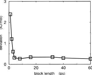
five independent windows extracted from the trajectory, on the size of the window. The 300 ps simulation of the Sbstate was
used in this analysis. Irrespective of the size of the window, the starting points for each window were chosen at 60 ps intervals. This made the data in each window as independent as possible. Figure 9 shows that the standard deviation initially decreases rapidly as the length of sampling is increased, but after the window size has reached 5 ps it remains unchanged despite an extension of the sampling by a further order of magnitude.
The dependence of accuracy on sampling time is different for derivative-based methods such as thermodynamic integration. As pointed out by Smith et al.,7truncating the Taylor series at various orders is equivalent to replacing the probability density function of∆V with a smooth function. The new function gives
the same corresponding lower-order moments for ∆V as the
ones calculated from the simulation, but gives zero higher-order moments. It is this implicitly implemented smoothing procedure that distinguishes the Taylor expansion formulas from the direct application of the perturbation formula. In practice, simulation time is always finite. The sampled ensemble contains noise as well as systematic errors due to incomplete sampling. The perturbation formula results always reflect all sources of noise and error. Thus, although in the current context, where the aim is to obtain crude estimates for the change in free energy associated with a large number of mutations from a single simulation, the application of the perturbation formula is overall more general and more efficient than extrapolation based on a Taylor expansion, this does not mean that the application of the perturbation formula will yield the better estimate in all cases.8 It also does not mean that in free energy calculations using a series of intermediate states the use of the perturbation formula is necessarily preferable.
Conclusions
For the purpose of predicting changes in free energy from a single simulation, extrapolation based on applying the perturba-tion formula is overall more general and more efficient than extrapolation based on a Taylor series expansion. It has been shown that by directly applying the perturbation formula, results comparable to those from thermodynamic integration calcula-tions using multiple intermediate states can be obtained for mutations involving moderate charge rearrangements and changes in atom type. It has also been shown that the range of potential modifications can be extended to include the creation or deletion of atoms by biasing the sampling in the reference state. This can be achieved by the inclusion of soft interaction sites at positions where atoms are to be created or deleted. As has been stated previously,6,7 extrapolation methods based on a single simulation have the advantage that a large number of potential modifications can be investigated with a single calculation. Furthermore, as the extrapolation is based on an unperturbed ensemble the nature of the perturbation does not have to be predefined. Thus, predictions for specific mutations can be efficiently obtained by reanalysis of existing trajectories. There are of course limitations on the mutations that can be treated using this approach. The method is only proposed as a means of obtaining estimates for the difference in free energy for a wide range of derivatives of a reference compound rapidly from a single simulation. It is not a replacement for free energy calculations in general. Nevertheless, considering the scope of the modifications treated in the test examples we feel that the approach could hold considerable promise for use as a rapid, nonempirical means of screening large numbers of compounds to guide experimental planning in drug design, a task not practical using normal free energy calculations.
a
b
c
Figure 8. Probability density functions F(∆V). The pair of lines in
the right part of each figure corresponds toFAand the pair of lines in
the left part corresponds toFB. The solid curves are computed directly
from 300 ps simulations and the dashed curves are extrapolated using formula 13. A line without symbols indicates that the line is obtained (either directly or using formula 13) from a simulation of the A state, while a line with symbols indicates that it is obtained from a simulation
of the B state. (a, top) A state)Sa, B state)Sb; (b, middle) A state
)Sa, B state)p-methylphenol; (c, bottom) A state)Sb, B state)
p-methylphenol.
Figure 9. Standard deviation of the calculated free energy differences
between the Saand the Sbstates using five blocks of data from the 300
Acknowledgment. Financial support from the Huber-Kudlich Foundation (grant 2-89-100-91) is gratefully acknowl-edged.
References and Notes
(1) Beveridge, D. L.; DiCapua, F. M. Annu. ReV. Biophys. Biophys. Chem. 1989, 18, 431.
(2) Jorgensen, W. L. Chemtracts: Org. Chem. 1991, 4, 91 (3) van Gunsteren, W. F.; Beutler, T. C.; Fraternali, F.; King, P. M.; Mark, A. E. In Computer simulation of biomolecular systems, theoretical and experimental applications; van Gunsteren, W. F., Weiner, P. K., Wilkinson, A. J., Eds.; ESCOM Science Publishers; Leiden, The Nether-lands, 1993, Vol. 2, pp 315-348.
(4) Mitchell, M. J.; McCammon, J. A. J. Comput. Chem. 1991, 12, 271.
(5) Burger, M. T.; Armstrong, A.; Guarnieri, F.; McDonald, D. Q.; Still, W. C. J. Am. Chem. Soc. 1994, 116, 3593.
(6) Gerber, P. R.; Mark, A. E.; van Gunsteren, W. F. J. Computor-Aided Mol. Des. 1993, 7, 305.
(7) Smith, P. E.; van Gunsteren, W. F. J. Chem. Phys. 1994, 100, 577.
(8) Levy, R. M.; Belhadj, M.; Kitchen, D. B. J. Chem. Phys. 1991, 95, 3627.
(9) King, G.; Barford, R. A. J. Phys. Chem. 1993, 97, 8798. (10) Mark, A. E.; van Helden, S. P.; Smith, P. E.; Janssen, L. H. M.; van Gunsteren, W. F. J. Am. Chem. Soc. 1994, 116, 6293.
(11) Kirkwood, J. G. J. Chem. Phys. 1935, 3, 300. (12) Zwanzig, R. W. J. Chem. Phys. 1954, 22, 1420.
(13) Jorgensen, W.; Ravimohan, C. J. Chem. Phys. 1985, 83, 3050. (14) Mezei, M.; Beveridge, D. L. Ann. N.Y. Acad. Sci. 1986, 482, 1. (15) Cross, A. J. Chem. Phys. Lett. 1986, 128, 198.
(16) Beutler, T. C.; Mark, A. E.; van Schaik, R. C.; Gerber, P. R.; van Gunsteren, W. F. Chem. Phys. Lett. 1994, 222, 529.
(17) Berendsen, H. J. C.; Grigera, J. R.; Straatsma, T. P. J. Phys. Chem.
1987, 91, 6269.
(18) Berendsen, H. J. C.; Postma, J. P. M.; van Gunsteren, W. F.; Hermans, J. Intermolecular Forces; Pullman, B., Ed.; Reidel: Dordrecht, The Netherlands, 1981; pp 331-342 .
(19) van Gunsteren, W. F.; Berendsen, H. J. C. Groningen Molecular Simulation Library Manual; Biomos, University of Groningen, The Netherlands, 1987.