Full Terms & Conditions of access and use can be found at
http://www.tandfonline.com/action/journalInformation?journalCode=ubes20
Download by: [Universitas Maritim Raja Ali Haji] Date: 12 January 2016, At: 22:49
Journal of Business & Economic Statistics
ISSN: 0735-0015 (Print) 1537-2707 (Online) Journal homepage: http://www.tandfonline.com/loi/ubes20
Estimation With Many Instrumental Variables
Christian Hansen, Jerry Hausman & Whitney Newey
To cite this article: Christian Hansen, Jerry Hausman & Whitney Newey (2008) Estimation With Many Instrumental Variables, Journal of Business & Economic Statistics, 26:4, 398-422, DOI: 10.1198/073500108000000024
To link to this article: http://dx.doi.org/10.1198/073500108000000024
Published online: 01 Jan 2012.
Submit your article to this journal
Article views: 346
View related articles
Estimation With Many Instrumental Variables
Christian H
ANSENGraduate School of Business, University of Chicago, Chicago, IL 60637 (chansen1@chicagoGSB.edu)
Jerry H
AUSMANDepartment of Economics, Massachusetts Institute of Technology, Cambridge, MA 02139 (jhausman@mit.edu)
Whitney N
EWEYDepartment of Economics, Massachusetts Institute of Technology, Cambridge, MA 02139 (wnewey@mit.edu)
Using many valid instrumental variables has the potential to improve efficiency but makes the usual in-ference procedures inaccurate. We give corrected standard errors, an extension of Bekker to nonnormal disturbances, that adjust for many instruments. We find that this adjustment is useful in empirical work, simulations, and in the asymptotic theory. Use of the corrected standard errors in t-ratios leads to an as-ymptotic approximation order that is the same when the number of instrumental variables grows as when the number of instruments is fixed. We also give a version of the Kleibergen weak instrument statistic that is robust to many instruments.
KEY WORDS: Inference; Many instruments; Standard errors; Weak instruments.
1. INTRODUCTION
Empirical applications of instrumental variables estimation often give imprecise results. Using many valid instrumental variables can improve precision. For example, as we show, using all 180 instruments in the Angrist and Krueger (1991) schooling application gives tighter correct confidence intervals than using three instruments. An important problem with using many instrumental variables is that conventional asymptotic ap-proximations may provide poor apap-proximations to the sampling distributions of the resulting estimators. Two-stage least squares (2SLS) is well known to have large biases when many instru-ments are used. The limited information maximum likelihood (LIML henceforth) or Fuller (1977, FULL henceforth) estima-tors correct this bias, but the usual standard errors are too small. We give corrected standard errors (CSE) that improve upon the usual ones, leading to a better normal approximation to t-ratios under many instruments. The CSE are an extension of those of Bekker (1994) that allow for non-Gaussian distur-bances. We show that the normal approximation with FULL and CSE is asymptotically correct with nonnormal disturbances under a variety of many instrument asymptotics, including the many instrument sequence of Kunitomo (1980), Morimune (1983), and Bekker (1994) and the many weak instruments se-quence of Chao and Swanson (2002, 2003, 2004, 2005) and Stock and Yogo (2005b). We also find that there is no penalty for many instruments in the rate of approximation of the dis-tribution of t-ratios when the CSE are used and an additional condition is satisfied. That is, the rate at which the distribution of the t-ratio approaches its standard normal limit is the same as with a fixed number of instruments. In addition, we give a version of the Kleibergen (2002) test statistic that is valid under many instruments, as well as under weak instruments.
We carry out a wide range of simulations to check the asymp-totic approximations. We find that FULL with the CSE gives confidence intervals with actual coverage quite close to nom-inal. We also show that LIML with the CSE has identical as-ymptotic properties to FULL and performs quite well in our simulations, as in those of Hahn and Inoue (2002). Our results also demonstrate that the concentration parameter (which can
be estimated) provides a better measure of accuracy for stan-dard inference with FULL or LIML than the F-statistic,R2, or other statistics previously considered in the literature.
In relation to previous work, the CSE, the validity of Bekker (1994) standard errors under many weak instrument asymp-totics, the rate of approximation results, and our many instru-ment view of the Angrist and Krueger (1991) application ap-pear to be novel. The limiting distribution results build on pre-vious work. For many instrument asymptotics we generalize LIML results of Kunitomo (1980), Morimune (1983), Bekker (1994), and Bekker and van der Ploeg (2005) to FULL, distur-bances that are not Gaussian, and general instruments. Our re-sults also generalize recent rere-sults of Anderson, Kunitomo, and Matsushita (2005) to many weak instruments, who had gener-alized results from an earlier version of this article by relaxing a conditional moment restriction. We also combine and gen-eralize results of Chao and Swanson (2002, 2003, 2005) and Stock and Yogo (2005b) by relaxing some kurtosis restrictions of Chao and Swanson (2003) and allowing a wider variety of se-quences of instruments and concentration parameter than Stock and Yogo (2005b). Our theoretical results make use of some inequalities in Chao and Swanson (2004).
Hahn and Hausman (2002) gave a test for weak instruments and Hahn, Hausman, and Kuersteiner (2004) showed that FULL performs well under weak instruments. Also, the random ef-fects estimator of Chamberlain and Imbens (2004) leads to ac-curate inference with many instruments. Recently Andrews and Stock (2006) derived asymptotic power envelopes for tests un-der several cases of many weak instrument asymptotics with Gaussian disturbances. We consider cases where the square root of the number of instruments grows more slowly than the con-centration parameter. There it turns out that Wald tests using the CSE attain the power envelope. We also consider cases where the number of instruments grows as fast as the sample size, which is not covered by Andrews and Stock (2006).
© 2008 American Statistical Association Journal of Business & Economic Statistics October 2008, Vol. 26, No. 4 DOI 10.1198/073500108000000024
398
The remainder of the article is organized as follows. In the next section, we briefly present the model and estimators that we will consider. We reexamine the Angrist and Krueger (1991) study of the returns to schooling in Section 3 and give a variety of simulation results in Section 4. Section 5 contains asymptotic results and Section 6 concludes.
2. MODELS AND ESTIMATORS
The model we consider is given by
y
T×1=T×XGGδ×01+ u
T×1, X=ϒ+V,
where T is the number of observations, G is the number of right-side variables, ϒ is a matrix of observations on the re-duced form, andV is the matrix of reduced form disturbances. For the asymptotic approximations, the elements ofϒ will be implicitly allowed to depend onT, although we suppress de-pendence ofϒ onT for notational convenience. Estimation of
δ0will be based on aT×KmatrixZ of instrumental variable observations.
This model allows forϒto be a linear combination ofZ, that is,ϒ =Zπ for someK×Gmatrixπ. Furthermore, columns ofX may be exogenous, with the corresponding column ofV
being zero. The model also allows forZto be functions meant to approximate the reduced form. For example, letϒt′ andZt′
denote thetth row (observation) ofϒ andZ, respectively. We could have ϒt=f0(wt) be an unknown function of a vector
wtof underlying instruments andZt=(p1K(wt), . . . ,pKK(wt))′
for approximating functionspkK(w),such as power series or
splines. In this case linear combinations of Zt may
approxi-mate the unknown reduced form, for example, as in Donald and Newey (2001).
It is well known that variability ofϒ relative toV is impor-tant for the properties of instrumental variable (IV) estimators. ForG=1 this feature is well described by
μ2T=
T
t=1
ϒt2/E[Vt2].
This concentration parameter plays a central role in the theory of IV estimators. The distribution of the estimators depends on
μ2T,with the convergence rate being 1/μT and the accuracy of
the usual asymptotic approximation depending crucially on the size ofμ2T.
To describe the estimators, letP=Z(Z′Z)−Z′whereA− de-notes any symmetric generalized inverse of a symmetric matrix
A, that is,A− is symmetric and satisfies AA−A=A. We con-sider estimators of the form
ˆ
δ=(X′PX− ˆαX′X)−1(X′Py− ˆαX′y)
for some choice of αˆ. This class includes all of the familiar k-class estimators except the least squares estimator. Special cases of these estimators are two-stage least squares (2SLS), whereαˆ =0, and LIML, where αˆ = ˜α andα˜ is the smallest eigenvalue of the matrix(X¯′X¯)−1X¯′PX¯ for X¯ = [y,X]. FULL is also a member of this class of estimators, whereαˆ = [ ˜α− (1− ˜α)C/T]/[1−(1− ˜α)C/T] for some constant C. FULL
has moments of all orders, is approximately mean unbiased for
C=1, and is second-order admissible forC≥4 under standard large sample asymptotics.
For inference we consider an extension of the Bekker (1994) standard errors to nonnormality and estimators other than LIML. Letu(δ)=y−Xδ,σˆu2(δ)= ˆu(δ)′uˆ(δ)/(T−G),α(δ)˜ =
u(δ)′Pu(δ)/u(δ)′u(δ),ϒˆ = PX, X˜(δ) = X − ˆu(δ)(uˆ(δ)′X)/
ˆ
u(δ)′uˆ(δ),Vˆ(δ)=(I−P)X˜(δ),κT=Tt=1ptt2/K, τT =K/T,
ˆ
H(δ)=X′PX− ˜α(δ)X′X,
ˆB(δ)= ˆσu2(δ)
(1− ˜α(δ))2X˜(δ)′PX˜(δ)
+ ˜α(δ)2X˜(δ)′(I−P)X˜(δ),
ˆ
(δ)= ˆB(δ)+ ˆA(δ)+ ˆA(δ)′+ ˆB(δ),
ˆ
A(δ)=
T
t=1
(ptt−τT)ϒˆt
T
t=1 ˆ
ut(δ)2Vˆt(δ)/T
′
,
ˆ
B(δ)=K(κT−τT) T
t=1
(ut(δ)2− ˆσu2(δ))Vˆt(δ)Vˆt(δ)′
/[T(1−2τT+κTτT)].
The asymptotic variance estimator is given by ˆ
= ˆH−1ˆHˆ−1, Hˆ = ˆH(δ),ˆ ˆ = ˆ (δ).ˆ
Whenδˆis the LIML estimator, Hˆ−1ˆB(δ)ˆ Hˆ−1 is identical to
the Bekker (1994) variance estimator. The other terms inˆ ac-count for third and fourth moment terms that are present with some forms of nonnormality. In generalˆ is a “sandwich” for-mula, withHˆ being a Hessian term.
The variance estimatorˆ can be quite different than the usual oneσˆu2Hˆ−1even whenKis small relative toT.This occurs be-causeHˆ is close to the sum of squares of predicted values for the reduced form regressions and ˆB(δ) depends on sums of
squares of residuals. When the reduced form r-squared is small, the sum of squared residuals will tend to be quite large relative toHˆ, leading to ˆB(δ)being larger thanHˆ. In contrast, the
ad-justments for nonnormalityAˆ(δ)ˆ andBˆ(δ)ˆ will tend to be quite small whenK is small relative toT, which is typical in appli-cations. Thus we expect that in applied work the Bekker (1994) standard errors and CSE will often give very similar results. Also, Bekker (1994) standard errors will be consistent under many weak instrument asymptotics whereK/T goes to zero.
As shown by Dufour (1997), if the parameter set is allowed to include values whereϒ=0, then a correct confidence inter-val for a structural parameter must be unbounded with prob-ability 1. Hence, confidence intervals formed using the CSE cannot be correct. Also, under the weak instrument sequence of Staiger and Stock (1997), the CSE confidence intervals will not be correct, that is, they are not robust to weak instruments. These considerations motivate a statistic that is asymptotically correct with weak or many instruments.
Such a statistic can be obtained by modifying the Lagrange multiplier statistic of Kleibergen (2002) and Moreira (2001). For anyδlet
LM(δ)=u(δ)′PX˜(δ) (δ)ˆ −1X˜(δ)′Pu(δ).
This statistic differs from previous ones in using (δ)ˆ −1in the middle. Its validity does not depend on correctly specifying the
reduced form. The statisticLM(δ)will be asymptotically dis-tributed as χ2(G) when δ =δ0 under both many and weak instruments. Confidence intervals for δ0 can be formed from
LM(δ)by inverting it. Specifically, for the 1−αquantileqof aχ2(G)distribution, an asymptotic 1−αconfidence interval is {δ:LM(δ)≤q}. As recently shown by Andrews and Stock (2006), the conditional likelihood ratio test of Moreira (2003) is also correct with weak and many weak instruments, though apparently not under many instruments, whereKgrows as fast asT. For brevity we omit a description of this statistic and the associated asymptotic theory.
We suggest that the CSE are useful despite their lack of ro-bustness to weak instruments. Standard errors provide a simple measure of uncertainty associated with an estimate. The confi-dence intervals based onLM(δ)are more difficult to compute. Also, as we discuss below, the t-ratios for FULL based on the CSE provide a good approximation over a wide range of empir-ically relevant cases we considered. This observation might jus-tify viewing the parameter space as being bounded away from
ϒ=0,thus overcoming the strict Dufour (1997) critique. Or, one might simply view that our theoretical and simulation re-sults are relevant enough for applications to warrant using the CSE.
It does seem wise to check for weak instruments in practice. One could use the Hahn and Hausman (2002) test. One could also compare a Wald test based on the CSE with a test based on
LM(δ). One could also develop versions of the Stock and Yogo (2005a) tests for weak instruments that are based on the CSE.
Because the concentration parameter is important for the properties of the estimators it is useful to have an estimate of it for the common case with one endogenous right-side variable. ForG=1 letσˆV2= ˆV′Vˆ/(T−K). An estimator ofμ2T is
ˆ
μT2= ˆX′Xˆ/σˆV2−K=K(Fˆ−1),
where Fˆ =(Xˆ′Xˆ/K)/[ ˆV′Vˆ/(T −K)] is the reduced form F-statistic. This estimator is consistent in the sense that under many instrument asymptotics
ˆ
μ2T μ2T
p
−→1.
In the general case with one endogenous right-side and other exogenous right-side variables we take
ˆ
μ2T=(K−G+1)(F˜−1),
whereF˜ is the reduced form F-statistic for the variables inZ
that are excluded fromX.
3. QUARTER OF BIRTH AND RETURNS TO SCHOOLING
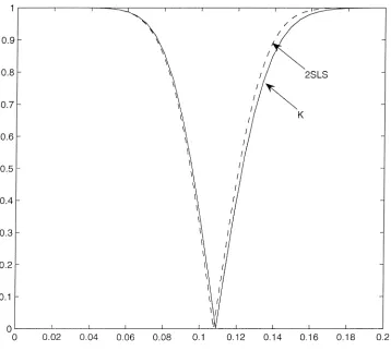
A motivating empirical example is provided by the Angrist and Krueger (1991) study of the returns to schooling using quar-ter of birth as an instrument. We consider data drawn from the 1980 U.S. Census for males born in 1930–1939. The model in-cludes a constant and year and state dummies. We report re-sults for 3 instruments and for 180 instruments. Figures 1–4 are graphs of confidence intervals at different significance levels using several different methods. The confidence intervals we consider are based on 2SLS with the usual (asymptotic)
stan-dard errors, FULL with the usual stanstan-dard errors, and FULL with the CSE. We take as a standard of comparison our ver-sion of the Kleibergen (2002) confidence interval (denoted K in the graphs), which is robust to weak instruments, many instru-ments, and many weak instruments.
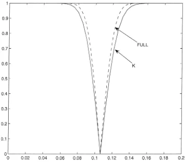
Figure 1 shows that with three excluded instruments (two overidentifying restrictions), 2SLS and K intervals are very similar. The main difference seems to be a slight horizontal shift. Because the K intervals are centered about the LIML esti-mator, this shift corresponds to a slight difference in the LIML and 2SLS estimators. This difference is consistent with 2SLS having slightly higher bias than LIML. Figure 2 shows that with 180 excluded instruments (179 overidentifying restrictions), the confidence intervals are quite different. In particular, there is a much more pronounced shift in the 2SLS location, as well as smaller dispersion. These results are consistent with a larger bias in 2SLS resulting from many instruments.
Figure 3 compares the confidence interval for FULL based on the usual standard error formula for 180 instruments with the K interval. Here we find that the K interval is wider than the usual one. In Figure 4, we compare FULL with CSE to K, finding that the K interval is nearly identical to the one based on the CSE.
Comparing Figures 1 and 4, we find that the CSE interval with 180 instruments is substantially narrower than the inter-vals with 3 instruments. Thus, in this application we find that using the larger number of instruments leads to more precise inference, as long as FULL and the CSE are used. These graphs are consistent with direct calculations of estimates and standard errors. The 2SLS estimator with 3 instruments is .1077 with standard error .0195 and the FULL estimator with 180 instru-ments is .1063 with CSE .0143. A precision gain is evident in the decrease in the CSE obtained with the larger number of instruments. These results are also consistent with Donald and Newey’s (2001) finding that using 180 instruments gives smaller estimated asymptotic mean square error for LIML than using just 3. Furthermore, Cruz and Moreira (2005) also found that 180 instruments are informative when extra covariates are used.
We also find that the CSE and the standard errors of Bekker (1994) are nearly identical in this application. Adding signif-icant digits, with 3 instruments the CSE is.0201002 whereas the Bekker (1994) standard error is.0200981, and with 180 in-struments the CSE is.0143316 and the Bekker (1994) standard error is.0143157. They are so close in this application because even when there are 179 overidentifying restrictions, the num-ber of instruments is very small relative to the sample size.
These results are interesting because they occur in a widely cited application. However, they provide limited evidence of the accuracy of the CSE because they are only an example. They re-sult from one realization of the data, and so could have occurred by chance. Real evidence is provided by a Monte Carlo study.
We based the study on the application to help make it em-pirically relevant. The design uses the same sample size as the application, and we fixed values for the instrumental variables and other exogenous variables at the sample values, for exam-ple, as in Staiger and Stock’s (1997) design for dummy variable instruments. The data were generated from a two-equation tri-angular simultaneous equations system with structural equation
Figure 1. Three instruments: K and 2SLS.
Figure 2. 180 instruments: K and 2SLS.
Figure 3. 180 instruments: K and Fuller.
Figure 4. 180 instruments: K and Fuller with Bekker standard errors.
as in the empirical application and a reduced form consisting of a regression of schooling on all of the instruments, including the covariates from the structural equation. The structural pa-rameters were set equal to their LIML estimated values from the 3 instruments case. The disturbances were homoscedastic Gaussian with (bivariate) variance matrix for each observation equal to the estimate from the application. Because the design has parameters equal to estimates, this Monte Carlo study could be considered a parametric bootstrap.
We carried out two experiments, one with 3 excluded instru-ments and one with 180 excluded instruinstru-ments. In each case the reduced form coefficients were set so that the concentration pa-rameter for the excluded instruments was equal to the unbiased estimator from the application. With 3 excluded instruments the concentration parameter value was set equal to the value of the consistent estimatorμˆ2T=95.6 from the data and with 180 ex-cluded instruments the value was set toμˆ2T=257.
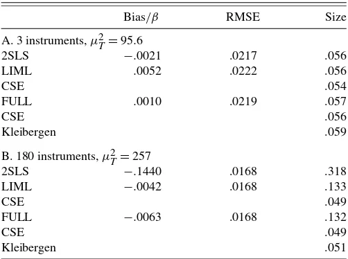
Table 1 reports the results of this experiment, giving relative bias, mean square error, and rejection frequencies for nominal 5% level tests concerning the returns to schooling coefficient. Similar results hold for the median and interquartile range. We are primarily interested in accuracy of inference and not in whether confidence intervals are close to each other, as they are in the application, so we focus on rejection frequencies. We find that with 3 excluded instruments all of rejection frequen-cies are quite close to their nominal values, including those for 2SLS. We also find that with 180 instruments, the significance levels of the standard 2SLS, LIML, and FULL tests are quite far from their nominal values, but that with CSE the LIML and FULL confidence intervals have the right level. Thus, in this Monte Carlo study we find evidence that using CSE takes care of whatever inference problem might be present in these data.
These results provide a somewhat different view of the An-grist and Krueger (1991) application than do Bound, Jaeger, and Baker (1996) and Staiger and Stock (1997). They viewed the 180 instrument case as aweakinstrument problem, appar-ently due to the low F-statistic, of about 3, for the excluded instruments. In contrast, we find that correcting formany instru-ments, by using FULL with CSE, fixes the inference problem.
Table 1. Simulation results
Bias/β RMSE Size A. 3 instruments,μ2T=95.6
2SLS −.0021 .0217 .056 LIML .0052 .0222 .056
CSE .054
FULL .0010 .0219 .057
CSE .056
Kleibergen .059 B. 180 instruments,μ2T=257
2SLS −.1440 .0168 .318 LIML −.0042 .0168 .133
CSE .049
FULL −.0063 .0168 .132
CSE .049
Kleibergen .051
NOTE: Males born 1930–1939. 1980 IPUMST=329,509,β=.0953.
We would not tend to find this result with weak instruments, because CSE do not correct for weak instruments as illustrated in the simulation results below. These results are reconciled by noting that a low F-statistic does not mean that FULL with CSE is a poor approximation. As we will see, a better criterion for LIML or FULL is the concentration parameter. In the Angrist and Krueger (1991) application we find estimates of the concen-tration parameter that are quite large. With 3 excluded instru-mentsμˆ2T=95.6 and with 180 excluded instrumentsμˆ2T=257. Both of these are well within the range where we find good performance of FULL and LIML with CSE in the simulations reported below.
4. SIMULATIONS
To gain a broader view of the behavior of LIML and FULL with the CSE we consider the weak instrument limit of the FULL and LIML estimators and t-ratios with CSE under the Staiger and Stock (1997) asymptotics. This limit is obtained by letting the sample size go to infinity while holding the con-centration parameter fixed. The limits of CSE and the Bekker (1994) standard errors coincide under this sequence because
K/T−→0. As shown in Staiger and Stock (1997), these limits provide excellent approximations to small sample distributions. Furthermore, it seems very appropriate for microeconometric settings, where the sample size is often quite large relative to the concentration parameter.
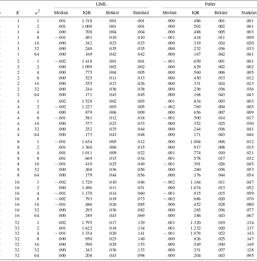
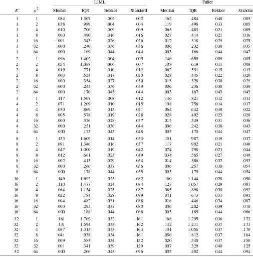
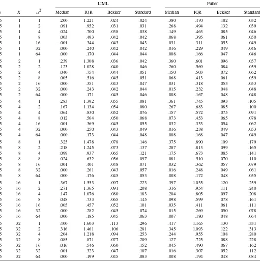
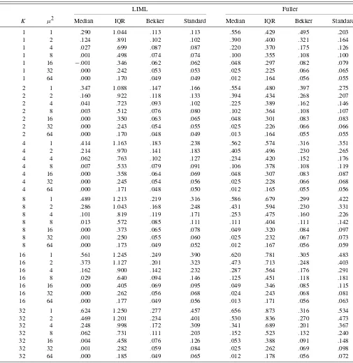
Tables 2–5 give results for the median, interquartile range, and rejection frequencies for nominal 5% level tests based on the CSE and the usual asymptotic standard error for FULL and LIML, for a range of numbers of instruments K; concentration parametersμ2T; and values of the correlation coefficientρ be-tweenutandVt. These three parameters completely determine
the weak instrument limiting distribution of t-ratios. Tables 2–5 give results forρ=0,ρ=.2,ρ=.5, andρ=.8, respectively. Each table contains results for several different numbers of in-struments and values of the concentration parameter.
Looking across the tables, there are a number of striking re-sults. We find that LIML is nearly median unbiased for small values of the concentration parameter in all cases. This bias does increase somewhat inρ andK, but even in the most ex-treme case we consider, with ρ=.8 and K=32, the bias is virtually eliminated with a μ2 of 16. Also, the bias is small whenμ2is 8 in almost every case. When we look at FULL, we see that it is more biased than LIML but that it is considerably less dispersed. The difference in dispersion is especially pro-nounced for low values of the concentration parameter, though FULL is less dispersed than LIML in all cases.
The results for rejection frequencies are somewhat less clear-cut than the results for size and dispersion. In particular, the re-jection frequencies tend to depend much more heavily on the value of K and ρ than do the results for median bias or dis-persion. For LIML, the rejection frequencies when the CSE are used are quite similar to the rejection frequencies when the usual asymptotic variance is used for small values ofK, but the CSE perform much better for moderate and large K, indicat-ing that usindicat-ing the CSE with LIML will generally be preferable. FULL with CSE performs better in some cases and worse in others than FULL with the conventional standard errors when
Table 2. Weak instrument limit of LIML and Fuller—ρ=0
LIML Fuller
ρ K μ2 Median IQR Bekker Standard Median IQR Bekker Standard 0 1 1 .001 1.318 .001 .001 .000 .486 .001 .001 0 1 2 .001 1.000 .001 .001 .000 .502 .002 .001 0 1 4 .000 .708 .004 .004 .000 .488 .005 .003 0 1 8 −.001 .491 .010 .010 −.001 .418 .011 .009 0 1 16 .000 .342 .023 .023 .000 .319 .024 .020 0 1 32 .000 .240 .035 .035 .000 .232 .036 .033 0 1 64 .000 .169 .042 .042 .000 .167 .042 .041 0 2 1 −.002 1.418 .001 .001 −.001 .659 .001 .001 0 2 2 .000 1.099 .002 .002 .000 .629 .002 .002 0 2 4 .000 .775 .004 .005 .000 .560 .006 .005 0 2 8 .000 .525 .011 .013 .000 .450 .013 .012 0 2 16 .000 .355 .023 .026 .000 .331 .024 .023 0 2 32 .000 .244 .036 .038 .000 .236 .036 .036 0 2 64 .000 .171 .043 .045 .000 .168 .043 .043 0 4 1 .002 1.528 .002 .003 .001 .834 .003 .003 0 4 2 −.002 1.227 .003 .005 −.002 .769 .004 .005 0 4 4 .000 .879 .006 .009 .000 .656 .007 .009 0 4 8 −.001 .581 .012 .018 −.001 .500 .014 .017 0 4 16 .000 .377 .023 .033 .000 .352 .025 .030 0 4 32 .000 .252 .035 .044 .000 .244 .036 .041 0 4 64 .000 .173 .043 .048 .000 .171 .043 .046 0 8 1 −.001 1.634 .005 .012 .000 1.004 .006 .012 0 8 2 .001 1.360 .006 .015 .000 .917 .008 .015 0 8 4 .001 1.011 .009 .022 .001 .774 .010 .021 0 8 8 .001 .669 .015 .034 .001 .578 .017 .032 0 8 16 −.001 .419 .025 .049 −.001 .391 .026 .045 0 8 32 .000 .268 .036 .056 .000 .260 .036 .053 0 8 64 .000 .179 .044 .056 .000 .176 .044 .054 0 16 1 −.002 1.720 .010 .046 −.002 1.164 .011 .047 0 16 2 .000 1.496 .011 .051 .000 1.074 .013 .052 0 16 4 −.001 1.170 .014 .060 −.001 .915 .015 .059 0 16 8 −.002 .793 .019 .073 −.002 .686 .020 .070 0 16 16 −.001 .486 .026 .085 .000 .452 .028 .080 0 16 32 .000 .295 .036 .082 .000 .285 .036 .077 0 16 64 .000 .189 .043 .069 .000 .186 .043 .067 0 32 1 .002 1.795 .017 .129 .001 1.320 .019 .134 0 32 2 .001 1.622 .018 .134 .001 1.232 .020 .137 0 32 4 −.001 1.334 .020 .141 −.001 1.076 .022 .143 0 32 8 .000 .950 .023 .149 .000 .826 .025 .147 0 32 16 .000 .590 .029 .153 .000 .549 .030 .149 0 32 32 .000 .343 .036 .133 .000 .331 .037 .128 0 32 64 .000 .208 .043 .098 .000 .204 .043 .095
K is small but clearly dominates forK large. The results also show that for small values of ρ, the rejection frequencies for LIML and FULL tend to be smaller than the nominal value, whereas the frequencies tend to be larger than the nominal value for large values ofρ.
An interesting and useful result is that both LIML and FULL with the CSE perform reasonably well for all values ofKandρ
in cases where the concentration parameter is 32 or higher. In these cases, the rejection frequency for LIML varies between .035 and .06, and the rejection frequency for FULL varies be-tween .035 and .070. These results suggest that the use of LIML or FULL with the CSE and the asymptotically normal approxi-mation should be adequate in situations where the concentration
parameter is around 32 or greater, even though in many of these cases the F-statistic takes on small values.
These results are also consistent with recent Monte Carlo work of Davidson and MacKinnon (2006). From careful examination of their graphs it appears that with few in-struments the bias of LIML is very small once the con-centration parameter exceeds 10, and that the variance of LIML is quite small once the concentration parameter ex-ceeds 20.
To see which cases might be empirically relevant, we sum-marize values ofKand estimates ofμ2andρ from some em-pirical studies. We considered all microeconomic studies that contain sufficient information to allow estimation of these
Table 3. Weak instrument limit of LIML and Fuller—ρ=.2
LIML Fuller
ρ K μ2 Median IQR Bekker Standard Median IQR Bekker Standard .2 1 1 .084 1.307 .002 .002 .162 .484 .048 .003 .2 1 2 .038 .989 .004 .004 .119 .498 .033 .005 .2 1 4 .010 .706 .009 .009 .065 .483 .021 .009 .2 1 8 .000 .490 .016 .016 .027 .414 .021 .016 .2 1 16 −.001 .343 .026 .026 .012 .318 .029 .025 .2 1 32 .000 .240 .036 .036 .006 .232 .038 .035 .2 1 64 .000 .169 .044 .044 .003 .166 .044 .042 .2 2 1 .096 1.402 .004 .005 .146 .650 .009 .005 .2 2 2 .054 1.088 .006 .007 .108 .619 .011 .008 .2 2 4 .019 .771 .010 .012 .062 .551 .015 .013 .2 2 8 .003 .524 .017 .020 .028 .445 .022 .020 .2 2 16 .000 .354 .027 .030 .013 .328 .030 .029 .2 2 32 .000 .244 .036 .039 .006 .236 .038 .038 .2 2 64 .000 .170 .043 .044 .003 .167 .043 .043 .2 4 1 .117 1.507 .008 .012 .146 .821 .012 .014 .2 4 2 .071 1.209 .010 .015 .108 .756 .014 .017 .2 4 4 .030 .869 .013 .021 .064 .642 .018 .022 .2 4 8 .005 .578 .019 .028 .028 .492 .023 .028 .2 4 16 .000 .376 .028 .037 .013 .349 .031 .036 .2 4 32 .000 .251 .036 .044 .006 .242 .038 .043 .2 4 64 .000 .173 .043 .048 .003 .170 .044 .047 .2 8 1 .133 1.609 .014 .033 .151 .987 .019 .037 .2 8 2 .091 1.346 .016 .037 .117 .902 .021 .040 .2 8 4 .047 1.000 .019 .042 .074 .758 .023 .044 .2 8 8 .012 .661 .023 .049 .034 .565 .027 .049 .2 8 16 .002 .415 .029 .054 .014 .386 .032 .053 .2 8 32 .000 .266 .037 .056 .006 .257 .038 .054 .2 8 64 .000 .178 .044 .055 .003 .175 .044 .054 .2 16 1 .149 1.692 .023 .082 .160 1.144 .028 .090 .2 16 2 .110 1.477 .024 .084 .127 1.057 .029 .091 .2 16 4 .064 1.154 .025 .087 .085 .898 .030 .092 .2 16 8 .022 .784 .028 .089 .041 .673 .031 .091 .2 16 16 .004 .482 .031 .088 .016 .446 .034 .087 .2 16 32 .000 .293 .037 .080 .006 .282 .039 .078 .2 16 64 .000 .188 .044 .068 .003 .185 .044 .066 .2 32 1 .161 1.769 .032 .161 .168 1.295 .036 .172 .2 32 2 .131 1.594 .033 .162 .142 1.211 .037 .171 .2 32 4 .087 1.313 .033 .163 .101 1.056 .037 .170 .2 32 8 .041 .938 .034 .161 .056 .812 .037 .164 .2 32 16 .009 .583 .034 .152 .020 .540 .037 .150 .2 32 32 .001 .341 .039 .129 .007 .329 .040 .125 .2 32 64 .000 .206 .043 .096 .003 .202 .044 .094
tities found in the March 1999 to March 2004American Eco-nomic Review, the February 1999 to June 2004Journal of Polit-ical Economy, and the February 1999 to February 2004 Quar-terly Journal of Economics. We found that 50% of the articles had at least one overidentifying restriction, 25% had at least three, and 10% had seven or more. As we have seen, the CSE can provide a substantial improvement even with small num-bers of overidentifying restrictions, so there appears to be wide scope for applying these results. Table 6 summarizes estimates ofμ2andρfrom these studies.
It is interesting to note that nearly all of the studies had val-ues ofρthat were quite low, so that theρ=.8 case considered above may not be very relevant for practice. Also, the
concen-tration parameters were mostly in the range where the many instrument asymptotics with CSE should work well.
5. MANY INSTRUMENT ASYMPTOTICS
Theoretical justification of the CSE is provided by asymp-totic theory where the number of instruments grows with the sample size and using the CSE in t-ratios leads to a better as-ymptotic approximation (by the standard normal) than do the usual standard errors. This theory is consistent with the empir-ical and Monte Carlo results where the CSE improve accuracy of the Gaussian approximation.
Table 4. Weak instrument limit of LIML and Fuller—ρ=.5
LIML Fuller
ρ K μ2 Median IQR Bekker Standard Median IQR Bekker Standard .5 1 1 .200 1.221 .024 .024 .380 .470 .182 .032 .5 1 2 .091 .952 .031 .031 .268 .494 .132 .039 .5 1 4 .024 .700 .038 .038 .149 .463 .085 .046 .5 1 8 .003 .493 .042 .042 .068 .395 .061 .050 .5 1 16 −.001 .344 .043 .043 .031 .311 .053 .049 .5 1 32 .000 .240 .042 .042 .016 .229 .049 .046 .5 1 64 .000 .170 .044 .044 .008 .166 .047 .046 .5 2 1 .239 1.308 .036 .042 .360 .601 .096 .057 .5 2 2 .123 1.028 .040 .046 .260 .569 .084 .059 .5 2 4 .040 .754 .044 .051 .150 .503 .072 .062 .5 2 8 .005 .516 .045 .051 .068 .413 .061 .059 .5 2 16 .000 .351 .043 .047 .031 .318 .053 .053 .5 2 32 .000 .243 .042 .044 .015 .232 .048 .048 .5 2 64 .000 .171 .045 .046 .008 .167 .048 .048 .5 4 1 .283 1.392 .055 .081 .361 .745 .093 .105 .5 4 2 .167 1.134 .054 .080 .267 .683 .085 .100 .5 4 4 .064 .830 .052 .076 .157 .572 .075 .091 .5 4 8 .012 .564 .050 .068 .073 .453 .065 .078 .5 4 16 .001 .369 .045 .055 .032 .333 .054 .062 .5 4 32 .000 .250 .043 .049 .016 .238 .049 .053 .5 4 64 .000 .173 .044 .048 .008 .168 .047 .049 .5 8 1 .325 1.478 .078 .146 .375 .890 .109 .179 .5 8 2 .218 1.245 .073 .137 .287 .813 .099 .165 .5 8 4 .099 .937 .065 .121 .175 .673 .085 .141 .5 8 8 .024 .632 .056 .097 .081 .510 .070 .110 .5 8 16 .001 .401 .048 .071 .032 .362 .057 .079 .5 8 32 .000 .261 .043 .057 .016 .248 .049 .061 .5 8 64 .000 .176 .045 .053 .008 .172 .048 .055 .5 16 1 .367 1.553 .097 .223 .397 1.035 .120 .259 .5 16 2 .271 1.365 .091 .208 .316 .954 .111 .240 .5 16 4 .147 1.076 .080 .183 .204 .805 .097 .208 .5 16 8 .048 .733 .065 .145 .098 .599 .078 .161 .5 16 16 .005 .457 .052 .101 .035 .411 .061 .111 .5 16 32 .000 .282 .045 .074 .015 .269 .050 .078 .5 16 64 .000 .185 .045 .063 .007 .180 .048 .064 .5 32 1 .400 1.603 .113 .296 .417 1.165 .130 .331 .5 32 2 .316 1.461 .106 .281 .345 1.093 .122 .313 .5 32 4 .204 1.218 .094 .253 .244 .955 .108 .280 .5 32 8 .085 .871 .077 .209 .127 .725 .088 .228 .5 32 16 .016 .546 .060 .152 .045 .490 .067 .162 .5 32 32 .001 .323 .047 .107 .016 .307 .052 .112 .5 32 64 .000 .199 .045 .083 .008 .194 .048 .084
Some regularity conditions are important for the results. Let Zt′,ut,Vt′, and ϒt′ denote the tth row of Z,u,V, and
ϒ, respectively. Here we will consider the case where Z is constant, leaving the treatment of random Z to future re-search.
Assumption 1. Z includes among its columns a vector of ones, rank(Z)=K,Tt=1(1−ptt)2/T≥C>0.
The restriction that rank(Z)=K is a normalization that re-quires excluding redundant columns from Z. It can be veri-fied in particular cases. For instance, whenwtis a continuously
distributed scalar,Zt=pK(wt), and pkK(w)=wk−1, it can be
shown that Z′Z is nonsingular with probability 1 for K<T.
[The observations w1, . . . ,wT are distinct with probability 1
and therefore, byK<T, cannot all be roots of aKth-degree polynomial. It follows that for any nonzero a there must be somet witha′Zt=a′pK(wt)=0, implying a′Z′Za>0.] The
conditionTt=1(1−ptt)2/T≥Cimplies thatK/T≤1−C,
be-causeptt≤1 impliesTt=1(1−ptt)2/T≤Tt=1(1−ptt)/T=
1−K/T.
Assumption 2. There is aG×GmatrixST= ˜STdiag(μ1T,
. . . , μGT) and zt such that ϒt =STzt/√T, S˜T is bounded
and the smallest eigenvalue of S˜TS˜T′ is bounded away from
zero, for each j either μjT =
√
T or μjT/
√
T −→0, μT =
min1≤j≤GμjT −→ ∞,and
√
K/μ2T −→0. Also, Tt=1 zt 4/
Table 5. Weak instrument limit of LIML and Fuller—ρ=.8
LIML Fuller
ρ K μ2 Median IQR Bekker Standard Median IQR Bekker Standard .8 1 1 .290 1.044 .113 .113 .556 .429 .495 .203 .8 1 2 .124 .891 .102 .102 .390 .400 .321 .164 .8 1 4 .027 .699 .087 .087 .220 .370 .175 .126 .8 1 8 .001 .498 .074 .074 .100 .355 .108 .100 .8 1 16 −.001 .346 .062 .062 .048 .297 .082 .079 .8 1 32 .000 .242 .053 .053 .025 .225 .066 .065 .8 1 64 .000 .170 .049 .049 .012 .164 .056 .055 .8 2 1 .347 1.088 .147 .166 .554 .480 .397 .275 .8 2 2 .160 .922 .118 .133 .394 .434 .268 .207 .8 2 4 .041 .723 .093 .102 .225 .389 .162 .146 .8 2 8 .003 .512 .076 .080 .102 .364 .108 .107 .8 2 16 .000 .350 .063 .065 .048 .301 .083 .083 .8 2 32 .000 .243 .054 .055 .025 .226 .066 .066 .8 2 64 .000 .170 .048 .049 .013 .164 .055 .055 .8 4 1 .414 1.163 .183 .238 .562 .574 .316 .351 .8 4 2 .214 .970 .141 .183 .405 .496 .230 .265 .8 4 4 .062 .763 .102 .127 .234 .420 .152 .176 .8 4 8 .007 .533 .079 .091 .106 .378 .108 .119 .8 4 16 .000 .358 .064 .069 .048 .307 .083 .087 .8 4 32 .000 .245 .054 .056 .025 .228 .066 .068 .8 4 64 .000 .171 .048 .050 .012 .165 .055 .056 .8 8 1 .489 1.213 .219 .316 .586 .679 .299 .422 .8 8 2 .286 1.043 .168 .248 .431 .594 .230 .331 .8 8 4 .101 .819 .119 .171 .253 .475 .160 .226 .8 8 8 .013 .572 .085 .111 .111 .404 .111 .142 .8 8 16 .000 .373 .065 .078 .049 .320 .084 .097 .8 8 32 .001 .250 .055 .060 .025 .232 .067 .073 .8 8 64 .000 .173 .049 .052 .012 .167 .056 .059 .8 16 1 .561 1.245 .249 .390 .620 .781 .305 .483 .8 16 2 .373 1.127 .201 .323 .473 .713 .248 .403 .8 16 4 .162 .900 .142 .232 .287 .564 .176 .291 .8 16 8 .029 .640 .094 .146 .125 .451 .118 .181 .8 16 16 .000 .405 .069 .095 .049 .346 .085 .115 .8 16 32 .000 .262 .056 .068 .024 .243 .068 .081 .8 16 64 .000 .177 .049 .056 .013 .171 .056 .063 .8 32 1 .624 1.250 .277 .457 .656 .873 .316 .534 .8 32 2 .469 1.201 .234 .401 .530 .836 .270 .473 .8 32 4 .248 .998 .172 .309 .341 .689 .201 .367 .8 32 8 .062 .731 .111 .203 .152 .523 .132 .240 .8 32 16 .004 .458 .076 .126 .053 .388 .091 .148 .8 32 32 .001 .282 .059 .084 .025 .262 .069 .098 .8 32 64 .000 .185 .049 .065 .012 .178 .056 .072
T2−→0,andTt=1ztz′t/T is bounded and uniformly
nonsin-gular.
This condition allows for both many instruments or many weak instruments. IfμT =
√
T, then K may grow as fast as
Tand still satisfy this condition. This case is many instruments.
Table 6. Five years of AER, JPE, QJE
Num. papers Median Q10 Q25 Q75 Q90
μ2 28 23.6 8.95 12.7 105 588
ρ 22 .279 .022 .0735 .466 .555
Allowing forK to grow and forμT to grow slower than
√
T
is the many weak instrument case. Assumption 2 will imply that, whenKgrows no faster thanμ2T, the convergence rate of
ˆ
δ will be no slower than 1/μT. WhenKgrows faster thanμ2T,
the convergence rate ofδˆwill be no slower than√K/μ2T. This condition allows for some components ofδto be weakly iden-tified and other components (like the constant) to be strongly identified.
Assumption 3. (u1,V1), . . . , (uT,VT) are independent with
E[ut] =0, E[Vt] =0, E[u8t] and E[ Vt 8] are bounded in t,
Var((ut,Vt′)′)=diag(∗,0), and∗is nonsingular.
This hypothesis includes moment existence and homoscedas-ticity assumptions. The consistency of the CSE depends on homoscedasticity, as does consistency of the LIML estimator itself with many instruments; see Bekker and van der Ploeg (2005), Chao and Swanson (2004), and Hausman, Newey, and Woutersen (2005).
Assumption 4. There is πKT such that 2T =
T t=1 zt −
πKTZt 2/T−→0.
This condition allows an unknown reduced form that is ap-proximated by a linear combination of the instrumental vari-ables. An important example is a model with
Xt=
π11Z1t+μTf0(wt)/
√
T Z1t
+ v0t
,
Zt=
Z1t
pK(wt)
,
where Z1t is a G2×1 vector of included exogenous vari-ables, f0(w) is a (G−G2) dimensional vector function of a fixed-dimensional vector of exogenous variables w and
pK(w)=def(p1K(w), . . . ,pK−G2,K(w))′. The variables inXtother
thanZ1tare endogenous with reduced formπ11Z1t+μTf0(wt)/
√
T. The functionf0(w)may be a linear combination of a sub-vector of pK(w), in which caseT =0 in Assumption 4, or
it may be an unknown function that can be approximated by a linear combination ofpK(w). ForμT =
√
T this example is like the model in Donald and Newey (2001) whereZtincludes
approximating functions for the optimal (asymptotic variance minimizing) instrumentsϒt, but the number of instruments can
grow as fast as the sample size. Whenμ2T/T−→0, it is a mod-ified version where the model is more weakly identmod-ified.
To see precise conditions under which the assumptions are satisfied, let
zt= f0(wt)
Z1t
,
ST= ˜STdiag(μT, . . . , μT,
√
T, . . . ,√T),
˜
ST=
I π11 0 I
.
By construction we haveϒt=STzt/
√
T. Assumption 2 imposes the requirements that
T
t=1
zt 4/T2−→0,
T
t=1
ztz′t/Tis uniformly nonsingular.
The other requirements of Assumption 2 are satisfied by con-struction. Turning to Assumption 3, we require that Var(ut,v′t)
is nonsingular. Because the submatrix ofS˜T corresponding to
Vtj=0 is the same as the submatrix corresponding to the
in-cluded exogenous variablesZ1t, we haveS˜T22=Iis uniformly nonsingular. For Assumption 4, let πKT = [ ˜πKT′ ,[IG2,0]′]′.
Then Assumption 4 will be satisfied if for eachT there exists ˜
πKTwith
2T =
T
t=1
zt−πKT′ Zt 2/T
=
T
t=1
f0(wt)− ˜πKT′ Zt 2/T−→0.
The following is a consistency result.
Theorem 1. If Assumptions 1–4 are satisfied andαˆ =K/T+ op(μ2T/T)orδˆ is LIML or FULL, thenμT−1S′T(δˆ−δ0)−→p0
andδˆ−→pδ0.
This result is more general than that in Chao and Swanson (2005) in allowing for strongly identified covariates but is simi-lar to that in Chao and Swanson (2003). See Chao and Swanson (2005) for an interpretation of the condition onαˆ. This result gives convergence rates for linear combinations ofδˆ. For in-stance, in the linear model example setup above, it implies that ˆ
δ1is consistent and thatπ11′ δˆ1+ ˆδ2=op(μT/
√
T).
Before stating the asymptotic normality results we describe their form. Letσu2=E[u2t],σVu2 =E[Vtut], γ =σVu/σu2,V˜ =
V−uγ′,having tth rowV˜t′; and let˜ =E[ ˜VtV˜t′]. There will
be two cases depending on the speed of growth ofKrelative to
μ2T.
Assumption 5. Either (I)K/μ2Tis bounded or (II)K/μ2T−→
∞.
To state a limiting distribution result it is helpful to also as-sume that certain objects converge. When considering the be-havior of t-ratios we will drop this condition.
Assumption 6. H = limT−→∞(1 − τT)z′z/T, τ =
limT−→∞τT, κ = limT−→∞κT, A = E[u2tV˜t] ×
limT−→∞Tt=1zt′(ptt − KT)/√KT exist and in case (I)
√
KS−T1−→S0or in case (II)μTS−T1−→ ¯S0.
Below we will give results for t-ratios that do not require this condition. LetB=(κ−τ )E[(u2t −σu2)V˜tV˜t′]. Then in case (I)
we will have
S′T(δˆ−δ0)
d
−→N(0, I),
S′TˆST p
−→I,
I=H−1 IH−1, (5.1)
I=(1−τ )σu2{H+S0˜S′0}
+(1−τ )(S0A+A′S′0)+S0BS′0. In case (II) we will have
(μT/
√
K)S′T(δˆ−δ0)
d
−→N(0, II),
(μ2T/K)S′TˆST p
−→II,
(5.2)
II=H−1 IIH−1,
II= ¯S0[(1−τ )σu2˜ +B]¯S′0.
The asymptotic variance expressions allow for the many in-strument sequence of Kunitomo (1980), Morimune (1983), and
Bekker (1994) and the many weak instrument sequence of Chao and Swanson (2003, 2005). This formula also extends that of Bekker and van der Ploeg (2005) to allow general instruments. WhenKandμ2T grow as fast asT, the variance formula gener-alizes that of Anderson et al. (2005), which had previously gen-eralized that of Hansen et al. (2004) to allow forE[ut| ˜Vt] =0
andE[u2t| ˜Vt] =σu2,to include the coefficients of included
ex-ogenous variables. The formula also generalizes that of Ander-son et al. (2005) to allow forμ2T andKto grow slower thanT. Thenτ =κ =0, A=0, andB=0, giving a formula which generalizes that of Stock and Yogo (2005b) to allow for in-cluded exogenous variables and to allow forK to grow faster thanμ2T, similarly to Chao and Swanson (2004). WhenKdoes grow faster thanμ2T, the asymptotic variance ofδˆmay be singu-lar. This occurs because the many instruments adjustment term is singular with included exogenous variables and it dominates the nonsingular matrixHwhenKgrows that fast.
Theorem 2. If Assumptions 1–6 are satisfied, αˆ = ˜α +
Op(1/T)or δˆis LIML or FULL, then in case (I) (5.1) is
sat-isfied and in case (II) (5.2) is satsat-isfied. Also, in each case, if is nonsingular, thenLM(δ0)−→dχ2(G).
It is straightforward to show that when the disturbances are Gaussian, the Wald test with the CSE attains the power enve-lope of Andrews and Stock (2006) under the conditions given here, where√K/μ2T−→0. Andrews and Stock (2006) showed that the LM statistic of Kleibergen (2002) attains this envelope and it is straightforward to show that the Wald statistic is as-ymptotically equivalent to the LM statistic under local alterna-tives. For brevity we omit this demonstration.
To give results for t-ratios and to understand better the per-formance of the CSE we now turn to approximation results. We will give order of approximation results for two t-ratios involv-ing linear combinations of coefficients, one with the CSE and another with the usual formula, and compare results.
We first give stochastic expansions around a normalized sum with remainder rate. To describe these results we need some additional notation. Define
ˆ
H=X′PX− ˆαX′X,
W= [(1−τT)ϒ+PZV˜ −τTV˜]S−T1′,
HT=(1−τT)z′z/T,
AT=
T
t=1
(ptt−τT)zt/
√
T
E[u2tV˜t′]S−T1′,
BT=(κT−τT)E[(ut2−σu2)V˜tV˜t′],
T=σu2(1−τT)(HT+KS−T1˜S−T1′)+(1−τT)(AT+A′T)
+KS−T1BTS−T1′,
T=HT−1 TH−T1.
We will consider t-ratios for a linear combination c′δˆ of the IV estimator, wherecare the linear combination coefficients, satisfying the following condition:
Assumption 7. There isμcT such that μTcc′S−T1′ is bounded and in case (I)(μcT)2c′S−T1′TS−T1cand(μcT)2c′S−
1′
T H−
1
T S−
1
T c
are bounded away from zero and in case (II)(μcT)2c′S−T1′T×
S−T1cμ2T/Kis bounded away from zero.
Letμ˜T=μT in case (I) andμ˜T=μ2T/
√
Kin case (II).
Theorem 3. Suppose that Assumptions 1–5 and 7 are satis-fied and αˆ = ˜α+Op(1/T)or δˆ is LIML or FULL. Then, for
εT=T+1/μ˜T in case (I) and case (II),
c′(δˆ−δ0)
c′ˆc
d
−→N(0,1),
c′(δˆ−δ0)
c′ˆc =
c′S−T1′HT−1W′u
c′S−T1′TS−T1c
+Op(εT).
Also, in case (II),
Prc′(δˆ−δ0)/
ˆ
σ2
uc′Hˆ−1c
≥C−→1
for allCwhereas in case (I),
c′(δˆ−δ0)
ˆ
σ2
uc′Hˆ−1c
= c′S
−1′
T H−
1
T W′u
σ2
uc′S−
1′
T H−
1
T S−
1
T c
+Op(εT).
Here we find that the t-ratio based on the linear combination
c′δˆ is equal to a sum of independent random variables, plus a remainder term that is of order 1/μ˜T+T. It is interesting to
note that in case (I) the rate of approximation is 1/μT+Tand
1/μT is the rate of approximation that would hold for fixedK.
For example, when μ2T =T andT =0, the rate of
approxi-mation is the usual parametric rate 1/√T. Thus, even whenK
grows as fast asT, the remainder terms in Theorem 3 can have the parametric 1/√Trate. This occurs because the specification ofW accounts for the presence of many instrumental variables. The reason that the t-ratio with the usual standard errors is unbounded whenK/μ2T −→ ∞is that the usual variance for-mula goes to zero relative to the full variance. WhenK grows that fast, the term that adjusts for many instruments asymptoti-cally dominates the usual variance formula.
To obtain approximation rates for the distribution of the nor-malized sums in the conclusion of Theorem 3, we impose the following restriction on the joint distribution ofutandVt.
Assumption 8. E[ut| ˜Vt] =0, E[u2t| ˜Vt] =σu2, E[|ut|4| ˜Vt] is
bounded, andTt=1 zt 3/T3/2=O(1/μT).
The vectorV˜t consists of residuals from the population
re-gression of Vt onut and so satisfiesE[ ˜Vtut] =0 by
construc-tion. Under joint normality of (ut,Vt),ut andV˜t are
indepen-dent, so the first two conditions automatically hold. In general, these two conditions weaken the joint normality restriction to first and second moment independence ofutfromV˜t. For
exam-ple, ifVt=γut+ ˜Vtfor anyV˜tthat is statistically independent
of ut, then Assumption 4 would be satisfied. The asymptotic
variance of the estimators is simpler under these conditions. This condition implies that E[u2tV˜t] =E[E[u2t| ˜Vt] ˜Vt] =0 and
E[u2tV˜tV˜t′] =E[E[u2t| ˜Vt] ˜VtV˜t′] =σu2E[ ˜VtV˜t′],so thatAT=0 and
BT=0.
Theorem 4. If Assumptions 1–5, 7, and 8 are satisfied, then for case (I)
Pr c
′S−1′
T H−
1
T W′u
c′S−T1′TS−T1c
≤q
=(q)+O(1/μT),
Pr c
′S−1′
T H−
1
T W′u
σ2
uc′S−
1′
T H−
1
T S−
1
T c
≤q
=(q)+O(1/μT+K/μ2T).
When the varianceT that adjusts for the presence of many
instruments appears in the denominator, the approximation is the fixedK rate 1/μT. In contrast, in case (I) when the usual
variance formulaσu2HT−1appears in the denominator, the rate of approximation has an additionalK/μ2T term. This term will go to zero more slowly than 1/μT whenK grows faster than
μT. WhenK grows as fast asμ2T, the remainder term does not
even go to zero, which corresponds to the usual standard errors being inconsistent.
We interpret this result as showing a clear advantage for the CSE with many instrumental variables. The condition for the usual standard errors to have as good an approximation rate as the CSE, thatKgrows slower thanμT,may not seem very
oner-ous whenμT=
√
T. However, whenμTgrows slower than
√
T
this condition would put severe limits on the number of instru-mental variables. Thus, if we think ofμT growing slowly as
representing a weakly identified model, we should expect to find an improvement from using the CSE even with small num-bers of instrumental variables. This interpretation is consistent with our empirical and Monte Carlo results.
It would be nice to combine Theorems 3 and 4 to obtain a re-sult on the rate of distributional approximation for the t-ratio. It is well known that this will hold with additional tail conditions on the remainder in the stochastic expansions of Theorem 3; see Rothenberg (1984). To do this is beyond the scope of this article.
We can also show that our modified version of the Kleibergen (2002) statistic is valid under weak instruments.
Theorem 5. If Assumptions 1–3 are satisfied, for eachj ei-ther μjT =1 or μjT =√T, and ST−1−→S0, Z′Z/T −→M, nonsingular, andZ′z/T−→R, thenLM(δ0)−→dχ2(G).
6. CONCLUSION
In this article, we have given standard errors that correct for many instruments when disturbances are not Gaussian. We have also shown that the LIML and Fuller (1977) estimators with Bekker (1994) standard errors provide improved inference rela-tive to the usual asymptotic approximation in instrumental vari-able settings across a wide range of applications. The Angrist and Krueger (1991) study provided an example where the CSE with 180 instruments is substantially smaller than the CSE with 3 instruments and confidence intervals closely match those of Kleibergen (2002). Through simulations, we confirm that us-ing the CSE leads to more accurate approximations in many cases. We also provide theoretical results that show the validity of the CSE under many instruments and under many weak in-struments without imposing normality. The theoretical results also show that the use of the CSE improves the approximation rate relative to when the usual standard errors are used. Overall, the results support the use of the CSE across a wide variety of applications.
ACKNOWLEDGMENTS
The NSF provided financial support for this article under grant 0136869. Amanda Kowalski provided excellent research assistance. Helpful comments were provided by A. Chesher, T. Rothenberg, J. Stock, and participants in seminars at Berkeley, Bristol, Cal Tech, Harvard–MIT, Ohio State, Stanford, the Uni-versity of Texas–Austin, UCL, and the UniUni-versity of Virginia.
APPENDIX: PROOFS OF THEOREMS
Throughout, letCdenote a generic positive constant that may be different in different uses and let M, CS, and T denote the conditional Markov inequality, the Cauchy–Schwarz inequality, and the triangle inequality, respectively.
Lemma A0. If Assumption 2 is satisfied and S′T(δˆ−δ0)/
μT 2/(1+ ˆδ 2)−→p0 then S′T(δˆ−δ0)/μT −→p0.
Proof. When ˆδ ≥adef=2 δ0 +(1+2 δ0 2)1/2,by sub-tracting 2 δ0 and squaring we have
( ˆδ −2 δ0 )2= ˆδ 2−4 ˆδ δ0 +4 δ0 2 ≥1+2 δ0 2.
Subtracting 2 δ0 2, adding ˆδ 2, and dividing by 2 gives
( ˆδ − δ0 )2≥(1+ ˆδ 2)/2.
By Assumption 2,λmin(STS′T/μ2T)≥C, so when ˆδ ≥a,
ST′(δˆ−δ0)/μT 2
1+ ˆδ 2 ≥C
ˆδ−δ0 2 1+ ˆδ 2 ≥C/2.
It follows that ˆδ <aw.p.a.1, and hence 1+ ˆδ 2<1+a2
and
S′T(δˆ−δ0)/μT 2≤(1+a2)
ST′(δˆ−δ0)/μT 2
1+ ˆδ 2
p
−→0.
Lemma A1. If conditional on theT×KmatrixZ, the obser-vations(ut,vt) (t=1, . . . ,T)are independent withE[ut|Z] =
E[vt|Z] =0, and there isCwithE[u4t] ≤C,E[v4t] ≤Cfor allt
then 1, then forP=Z(Z′Z)−Z′,
Var(u′Pv|Z)≤CK, u′Pv−E[u′Pv|Z] =Op(
√
K).
Proof. For notational simplicity we suppress the condition-ing onZ. Letσut2=E[u2t],σuvt=E[utvt], σvt2=E[v2t]. By
con-ditional independence of observations, E[uv′|Z] =diag(σuv1,
. . . , σuvT)
def
= Ŵ. Then E[u′Pv|Z] = tr(PE[vu′]) =tr(PŴ) =
T
t=1pttσuvt, wherepst=Pst. Then we have
E[(u′Pv)2|Z]
=
T
r,s,t,w=1
prsptwE[urvsutvw]
=
t
p2ttE[u2tv2t] +
s=t
{(pssptt+p2st)σuvsσuvt+p2stσus2σvt2}
=
t
p2tt{E[u2tv2t] −2σuvt2 −σus2σvt2} +
s,t
psspttσuvsσuvt
+
The second conclusion follows by M.
Lemma A2. If (i) P is a constant idempotent matrix with rank(P)=K; (ii) (W1T,V1,u1), . . . , (W1T,VT,uT) are
inde-where we suppress theTsubscript onvtfor convenience. Then
we have
Note that ytT is martingale difference, so that we can apply
a martingale central limit theorem. It follows by P idempo-tent that Ts=1p2st=ptt and Tt=1ptt =K. Then, for DT =
Note thats2T is bounded and bounded away from zero. Also
T satisfied. To apply the martingale central limit theorem it now suffices to show that forZt=(WtT,Vt,ut),
uj/
To finish showing that (A.1) is satisfied it only remains to show that for¯ytT=j<t(vtptjuj+vjptjut)/
Consider the last two terms. Note that
E
Also by lemma A2 of Chao and Swanson (2004),
Similar arguments can also be applied to show that each of the other four terms following the equality in (A.3) converges in probability to zero. It then follows by T and M that (A.3) is satisfied. By T it then follows that (A.1) is satisfied. Thus all the conditions of the Martingale central limit theorem are satisfied, so thatTt=2ytT−→dN(0,1). Then by the Slutzky theorem the
conclusion holds.
For the next result let S¯T =diag(μT,ST), X˜ = [u,X]¯S−T1′,
andHT=(1−τT)Tt=1ztz′t/T.
Lemma A2a. If Assumptions 1–4 are satisfied and √K/ μ2T−→0, then
LetAˆ= ˜X′PX˜−(K/T)X˜′X˜. Then by T, w.p.a.1,
Lemma A3. If Assumptions 1–4 are satisfied, then S′T ×
(δˆLIML−δ0)/μT−→p0. bounded matrix converges to zero; w.p.a.1 it follows that
C≤(1,−δ′)Bˆ(1,−δ′)′=(y−Xδ)′(y−Xδ)/T
Lemma A4. If Assumptions 1–4 are satisfied, then α˘ =
K/T+Op(