www.elsevier.com/locate/dsw
An analysis of multiple-class vacation queues with individual
thresholds
Ho Woo Lee
a;∗, Won Joo Seo
a, Seung Hyun Yoon
baDepartment of Systems Management Engineering, Sung Kyun Kwan University, Su Won, South Korea bETRI, Dae Jon, South Korea
Received 15 July 1998; received in revised form 1 August 2000
Abstract
This study examines a multiple-class M=G=1 queue with multiple thresholds. Each class of customer arrives according to an independent Poisson process, and each class has its own threshold. The idle server is reactivated as soon as any one of the thresholds is reached. Both FCFS and non-preemptive priority cases are considered. The Laplace–Stieltjes transform of the waiting time distribution function and the mean waiting time for each class of customers are derived. c 2001 Elsevier Science B.V. All rights reserved.
Keywords:Queues; Multiple class; Priority; N-policy
1. Introduction
Most studies on N-policy use a single threshold. This has been the tendency for studies involving multiple class queues. In these models, the idle server is reactivated when the total number of customers (including all classes) reaches a threshold (for an example of this, see [12]). In this paper a queueing system is proposed in which each class has its own threshold and the idle server is reactivated as soon as any one of the thresholds is reached. This paper was motivated by a real production system in which a machine needed to process multiple types of products.
The rst study on N-policy was carried out by Yadin and Naor [14]. They obtained the mean waiting time and the mean queue length, and then derived the optimal N∗ that minimizes the overall average operating cost. Hofri [4] studied two N-policy queues attended by a single server. Lee et al. [9] considered a threshold policy in which the server is reactivated when the number of the start-up class reached its threshold, regardless
∗Corresponding author.
E-mail address: [email protected] (H.W. Lee).
of the number of customers in other classes. For more studies on N-policy and related works, readers are advised to see Takagi [12].
The queueing system related to N-policy can be thought of as a vacation system. Vacation queues have attracted much attention from numerous researchers since Levy and Yechiali [10] and Heyman [3]. Kella [5] studied the M=G=1 queue with N-policy and vacations. Batch arrival queues under N-policy, with and without multiple vacations, were rst studied by Lee and Srinivasan [8]. Lee et al. [6,7] considered batch arrival queues with N-policy and vacations, and derived the queue length distribution in decomposed forms. The decomposition property was rst proved by Fuhrmann and Cooper [2] and then by Shanthikumar [11]. For a comprehensive survey on vacation queues, readers are advised to see Doshi [1] and Takagi [12].
2. The system and notation
A system with the following specications is considered in this study: (1) There are r classes.
(2) Customers of class p; (p= 1;2; : : : ; r) arrive according to a Poisson process with rate p independently
of other classes.
(3) Service times within a class are identically and independently distributed. Dierent classes have dierent service time distributions, but they are independent of each other.
(4) There is a single server and the queue capacity is unlimited.
(5) If no priorities are applied, FCFS is assumed regardless of the classes. If priorities are applied, non-preemption is assumed. Class-i has higher priority over class-j, fori ¡ j. FCFS is applied within a class. (6) Class-p has a threshold of Np.
(7) The idle server is reactivated as soon as any one of the thresholds is reached.
Let us dene the following notations. For the purpose of convenience, the test customer is assumed to belong to class-p. In most cases, the notations used by Takagi [12] are adopted, but some minor modications are made.
HC high-priority customer, i.e., a customer who belongs to one of the classes{1;2; : : : ; p−1}
EHC equal- or high-priority customer, i.e., a customer who belongs to one of the classes
{1;2; : : : ; p}
EC equal-priority customer, i.e., a customer belonging to class-p.
LC low-priority customer, i.e., a customer who belongs to one of the classes {p + 1; p+ 2; : : : ; r}
BPIP busy period initiation point
Wq∗(p)() the Laplace–Stieltjes transform (LST) of the distribution function (DF) of the waiting time of a class-p test customer
E(Wq(p)) mean waiting time of a class-p test customer
p arrival rate of class-p customers
=Pr
k=1k total arrival rate
+
p = Pp
k=1k arrival rate of EHCs
p−=Pr
k=p+1k arrival rate of LCs
Sp service time of a class-p customer (random variable)
Bp(x) = Pr(Sp6x); DF of Sp
B∗p() the LST of Bp(x)
B∗() = Pr
k=1(k=)B∗k(); the LST of the DF of the service time of a randomly selected
B+p∗() =Pp
k=1(k=+p)B∗k(); the LST of the DF of the service time of a randomly selected EHC
B−∗
p () =
Pr
k=p+1(k=p−)B∗k(); the LST of the DF of the service time of a randomly selected
LC
bp =E(Sp); the mean service time of a class-p customer.
b =Pr
k=1(k=)bk;the mean service time of a randomly selected customer from all classes
b(2)p =E(Sp2); the second moment of the service time of a class-p customer
b+
p =
Pp
k=1(k=+p)bk; the mean service time of a randomly selected EHC
b−p =Pr
k=p+1(k= −
p)bk; the mean service time of a randomly selected LC
p=pbp steady-state probability that the server is serving a class-p customer
=Pr
k=1k steady-state probability that the server is busy
+
p = Pp
k=1k steady-state probability that the server is serving an EHC
−p = Pr
k=p+1k steady-state probability that the server is serving an LC
+
p() =B+p∗[+p+−+p+p()]; the delay cycle generated by the service of an EHC and its
EHC-osprings
(i1; i2; : : : ; ir) a system state during the idle period in which there areik class-k customers, (06ik6Nk−
1; k= 1;2; : : : ; r)
R(i1; i2;:::; ir) the remaining idle period from an arbitrary time point in the state (i1; i2; : : : ; ir). From
PASTA (Wol [13]), this is equal to the remaining idle period under a condition where an arriving customer comes upon the state (i1; i2; : : : ; ir).
3. Analysis of the idle period
Before we derive the LST of the waiting time distribution of a class-p test customer, it is necessary to analyze the idle period.
First, the probability that the idle period visits state (i1; i2; : : : ; ir) is given by
(i1; i2;:::; ir)=
(i1+i2+· · ·+ir)!
i1!i2!: : : ir!
1
i1
2
i2
· · ·
r
ir
; (06ik6Nk−1; k= 1;2; : : : ; r): (1)
The mean staying time for the state (i1; i2; : : : ; ir) is 1= for any combination of i1; i2; : : : ; ir. Thus, the
steady-state probability that the system is in the state (i1; i2; : : : ; ir) under the condition that the system is idle
is given by
P(i1; i2;:::; ir)=
(i1; i2;:::; ir)
PN1−1
i1=0
PN2−1
i2=0 · · ·
PNr−1
ir=0 (i1; i2;:::; ir)
: (2)
From PASTA, it is also the probability that a test customer that arrives during the idle period encounters the state (i1; i2; : : : ; ir).
Now, let us obtain the LST of the DF of R(i1; i2;:::; ir). Under the event Aj that the rst arrival during
(i1; i2; : : : ; ir) is of class-j, we have
R(i1; i2;:::; ir)=Tj+R(i1;:::; ij+1;:::; ir); (3)
whereTj is the time until the rst arrival under Aj. It is easily seen thatTj follows the exponential distribution
the LST of the DF of R(i1; i2;:::; ir) is given by
R∗(i1; i2;:::; ir)() =
r X
j=1
j
T
∗
j()R∗(i1;:::; ij+1;:::; ir)(); (4a)
where
R∗(i1;:::; Nk−1;:::; ir)() =
k−1
X
j=1
j
T
∗
j()R∗(i1;:::; ij+1;:::; Nk−1;:::; ir)() +
k
T
∗
k()
+
r X
j=k+1
j
T
∗
j()R∗(i1;:::; Nk−1;:::; ij+1;:::; ir)() (4b)
and
R∗(N1−1; N2−1;:::; Nr−1)() =
r X
j=1
j
T
∗
j(): (4c)
The mean can be obtained recursively from
E(R(i1; i2;:::; ir)) =
r X
j=1
j
1
+E(R(i1;:::; ij+1;:::; ir))
; (5a)
where
E(R(i1;:::; Nk−1;:::; ir)) =
k−1
X
j=1
j
1
+E(R(i1;:::; ij+1;:::; Nk−1;:::; ir))
+
k
1
+
r X
j=k+1
j
1
+E(R(i1;:::; Nk−1;:::; ij+1;:::; ir))
(5b)
and
E(R(N1−1; N2−1;:::; Nr−1)) =
1
: (5c)
4. Waiting times under FCFS
In this section, we derive the LST of the distribution function of the waiting time of a class-ptest customer under FCFS. The server is busy with a probability of =Pr
k=1 k. Thus, the LST W ∗
q(p);FCFS() of the DF
of the waiting time of a class-p test customer can be written as
Wq∗(p);FCFS() =Wq∗(p);FCFS(|busy) + (1−)Wq∗(p);FCFS(|idle): (6)
To obtain Wq∗(p);FCFS(|busy) we need to nd the probability distribution for the number of customers at the busy period initiation point (BPIP). Let K(z1; z2; : : : ; zr) be the joint PGF (probability generating function)
of (7) is provided in the appendix).
The rst moment becomes
E(T0) =−
The second moment becomes
E(T02) = d
2
=
The busy period is a delay cycle with T0 as the initial delay. The LST of the distribution function of the
Fig. 1. Mean waiting time whenN1 varies (FCFS).
with mean
E(Wq(p);FCFS|busy) =
E(T02) 2E(T0)
+ b
(2)
2(1−): (10)
Under the FCFS discipline, the DFs of the waiting times of the customers that arrive during the busy period do not dier among classes. Thus (9) and (10) can be applied to all classes.
Now let us obtain the LST of the DF of the waiting time of the class-p test customer that arrives during the idle period. Let E(i1;:::; ir)(p) be the event that the class-p test customer encounters an idle state (i1; : : : ; ir)
when it arrives. Let w(∗i1;:::; ir)(p)() be the LST of the DF of the waiting time under E(i1;:::; ir)(p). Then we get
w∗(i1;:::; ir)(p)() = [B∗1()]i1: : :[B∗
r()]irR∗(i1;:::; ip+1;:::ir)(): (11)
From PASTA, we have
Wq∗(p);FCFS(|idle) =
N1−1
X
i1=0
· · · Nr−1
X
ir=0
P(i1;:::; ir)w ∗
(i1;:::; ir)(p)(); (12)
where P(i1;:::; ir) was obtained in (2). Unlike W ∗
q(p);FCFS(|busy); Wq∗(p);FCFS(|idle) depends on p. It can be
shown that the mean becomes
E(Wq(p); FCFS|idle) = N1−1
X
i1=0
· · · Nr−1
X
ir=0
P(i1;:::; ir)[i1b1+· · ·+irbr+E(R(i1;:::; ip+1;:::; ir))]: (13)
Using (9) and (12) in (6), we get
Wq∗(p);FCFS() =1−T
∗ 0()
E(T0)
(1−)
−+B∗() + (1−)
N1−1
X
i1=0
· · · Nr−1
X
ir=0
P(i1;:::; ir)w ∗
(i1;:::; ir)(p)(): (14)
The mean waiting time becomes
E(Wq(p);FCFS) =E(Wq(p);FCFS|busy) + (1−)E(Wq(p);FCFS|idle)
=
E(T02) 2E(T0)
+ b
(2)
2(1−)
+ (1−)
N1−1
X
i1=0
· · · Nr−1
X
ir=0
P(i1;:::; ir)[i1b1+· · ·+irbr+E(R(i1;:::; ip+1;:::; ir))]:
(15) The mean number of customers can be obtained from the Little’s law.
Fig. 2. Mean waiting time whenN3 varies (FCFS).
5. Waiting times under non-preemptive priority
In this section, we consider the waiting times in the case of non-preemptive priority (NP). We still have
Wq∗(p); NP() =Wq∗(p); NP(|busy) + (1−)Wq∗(p); NP(|idle): (16)
First, we obtain X(z), the PGF of the number of EHCs at the BPIP. This can be obtained by using z in place of z1; z2; : : : zp and by using 1 in zp+1; zp+2; : : : ; zr in (7):
X(z) =K(z1; z2; : : : ; zr)|z1=z2=···=zp=z; zp+1=zp+2=···=zr=1: (17)
Let T0(p) be the time that it takes to serve all EHCs existing at the BPIP and T0(∗p)() be its LST. Then
we get
T0(∗p)() =X[B+p∗()]: (18a)
The rst moment becomes
E(T0(p)) =−
d dT
∗
0(p)()|=0
=
1
N1
× Nr−1
X
ir=0
· · · N2−1
X
i2=0
(i2+· · ·+ir)!
i2!: : : ir!
N1+i2+· · ·+ir−1
i2+· · ·+ir
2
i2
· · ·
r
ir
(N1+i2+· · ·+ip)b+p+· · ·
+
p
Np
× Nr−1
X
ir=0
· · · Np+1−1
X
ip+1=0
Np−1−1
X
ip−1=0 · · ·
N1−1
X
i1=0
(i2+· · ·+ip−1+ip+1+· · ·+ir)!
i2!: : : ip−1!ip+1!: : : ir!
×
N1+i1+· · ·+ip−1+ip+1+· · ·+ir−1
i1+· · ·+ip−1+ip+1+· · ·+ir
×
1
i1
· · ·
p−1
ip−1 p+1
ip+1
· · ·
r
ir
+
The second moment becomes
×[(i1+· · ·+ip)(i1+· · ·+ip−1)(b+p)2+ (i1+· · ·+ip)b+(2)p ] +· · ·
+
r
Nr
× Nr−1−1
X
ir−1=0 · · ·
N1−1
X
i1=0
(i1+· · ·+ir−1)!
i1!: : : ir−1!
Nr+i1+· · ·+ir−1−1
i1+· · ·+ir−1
×
1
i1
· · ·
r−1
ir−1
×[(i1+· · ·+ip)(i1+· · ·+ip−1)(b+p)2+ (i1+· · ·+ip)b+(2)p ]: (18c)
The busy period is composed of two types of intervals:
(i) T0(p)-cycle: The time duration from the BPIP to the rst time when there are no EHC s. It is a delay
cycle which has T0(p) as the initial delay and is extended by EHCs and their EHC-osprings.
(ii) B−
p-cycle: A delay cycle that starts with the service of an LC (there are no EHC s at this point) and is
extended by its EHC-osprings. Let T0(p) and B−
p be the probabilities of the class-p test customer that arrives during the busy period and
nds T0(p)-cycle and B−p-cycle, respectively. Since every LC generates its own B−p-cycle, we get, after using
E(Bp−-cycle) = b
−
p
1−+
p !
;
B−
p = −
p
b−p
1−+
p !
=
−
p
1−+
p
: (19)
From T0(p)+B−
p =, we get
T0(p)=
+p(1−) 1−+
p
: (20)
We can apply the same delay-cycle argument that we employed in the FCFS case (Eq. (9)) and get
Wq∗(p); NP(|busy) =T0(p)
(1−+p)[1−T0(∗p)(p+−1)]
E(T0(p))[−p+pB∗p(+p−1)]
+B
−
p
(1−+p)[1−B−∗p (+p−1)]
E(Bp−)[−p+pB∗p(p+−1)]
;
(21) where +p−1=++p−1−+p−1+p−∗1() and p+−∗1() =B+p−∗1(+p−1). Note that+p−∗1() is a busy period that starts with the service of a HC and is extended by its HC-osprings.
The mean becomes
E(Wq(p); NP|busy) =
(1−)+
p
2(1−+p−1)(1−+
p)
E(T2 0(p))
E(T0(p))
+
+
pb
+(2)
p
1−+
p !
+
−
p
2(1−+p−1)(1−+
p)
b−p(2)
b−p
+
+
pb
+(2)
p
1−+
p !
: (22)
The waiting time of a class-p test customer that arrives during the idle period consists of (i) the remaining idle period,
(iii) the time it takes to serve all EC s that already exist at the arrival point of the test customer and their
is given by
w∗(i1;:::; ir)(p)() =∗(i1;:::; ip+1;:::; ir)(p)()[Bp∗(+p−1)]ip: (25)
Then we get
Wq∗(p);NP(|idle) =
The mean becomes
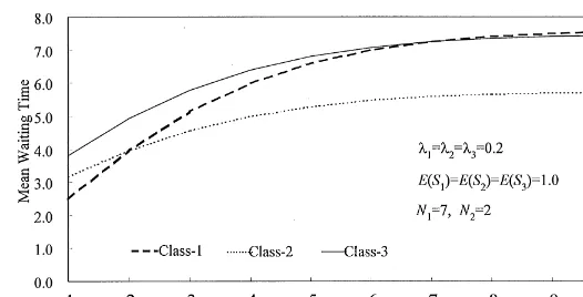
Fig. 3. Mean waiting time whenN1 varies (NP).
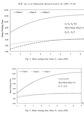
Fig. 4. Mean waiting time whenN3 varies (NP).
+ (1−)
N1−1
X
i1=0
· · · Nr−1
X
ir=0
P(i1; i2;:::; ir)
"
ipbp
1−+
p−1
+E((i1;:::; ip+1;:::; ir)(p)
#
: (28)
The mean number of customers can be obtained from the Little’s law.
Figs. 3 and 4 show the behavior of the mean waiting time when one of the thresholds varies while the other two are xed.
Acknowledgements
Appendix Derivation of Eq. (7)
Let us consider the case for three classes. The r-class case is a simple extension. Let TNp be the time until
Np class-p customers arrive. TNp follows the Erlang distribution with pdffNp(t) =
It suces to see the rst term on the right-hand side of (A.1). It becomes
N3−1
To evaluate the right-hand side of (A.2), we consider the following identity:
By replacing by 2+3 and k by n+m in (A.3), (A.2) becomes
Now using the identity
Thus (A.2) becomes
N3−1
Similar derivations can be applied to the second and third terms of (A.1) to get (7).
References
[1] B.T. Doshi, Queueing systems with vacations: a survey, Queueing Systems 1 (1986) 29–66.
[2] S.W. Fuhrmann, R.B. Cooper, Stochastic decompositions in the M=G=1 queue with generalized vacations, Oper. Res. 33 (5) (1985) 1117–1129.
[3] D.P. Heyman,T-policy for the M=G=1 queue, Management Sci. 23 (1977) 775–778.
[5] O. Kella, The threshold policy in the M=G=1 queue with server vacations, Naval Res. Logistics 36 (1989) 111–123.
[6] H.W. Lee, S.S. Lee, K.C. Chae, Operating Characteristics ofMXG=1 Queue withN-policy, Queueing Systems 15 (1994) 387–399. [7] H.W. Lee, S.S. Lee, J.O. Park, K.C. Chae, Analysis of MXG=1 Queue withN-policy and Multiple Vacations, J. Appl. Probab. 31
(1994) 467–496.
[8] H.S. Lee, M.M. Srinivasan, Control Policies for theMXG=1 Queueing System, Management Sci. 35 (6) (1989) 708–721. [9] H.W. Lee, S.H. Yoon, W.J. Seo, Start-up class models in multiple-class queues withN-policy, Queueing Systems 31 (1999) 101–124. [10] Y. Levy, Y. Yechiali, Utilization of Idle Time in an M=G=1 Queueing Systems, Management Sci. 22 (1975) 202–211.
[11] J.G. Shanthikumar, On stochastic decomposition in M=G=1 type queues with generalized server vacations, Oper. Res. 36 (4) (1988) 566–569.
[12] H. Takagi, Queueing Analysis, Vol. 1, North-Holland, Amsterdam, 1991.
[13] R.W. Wol, Poisson arrivals see time averages, Oper. Res. 30 (2) (1982) 223–231.