Blow-up of Solutions to a Periodic
Nonlinear Dispersive Rod Equation
Liangbing Jin, Yongming Liu, and Yong Zhou*
Received: November 12, 2009 Revised: April 6, 2010
Communicated by Heinz Siedentop
Abstract. In this paper, firstly we find an optimal constant for a convolution problem on the unit circle via the variational method. Then by using the optimal constant, we give a new and improved sufficient condition on the initial data to guarantee the corresponding strong solution blows up in finite time. We also analyze the cor-responding ordinary difference equation associate to the convolution problem and give numerical simulation for the optimal constant.
2010 Mathematics Subject Classification: Primary 30C70; Secondary 37L05, 35Q58, 58E35.
Keywords and Phrases: best constant, convolution problem, rod equa-tion, singularity.
1 Introduction
Although a rod is always three-dimensional, if its diameter is much less than the axial length scale, one-dimensional equations can give a good description of the motion of the rod. Recently Dai [16] derived a new (one-dimensional) nonlinear dispersive equation including extra nonlinear terms involving second-order and third-second-order derivatives for a compressible hyperelastic material. The equation reads
vτ+σ1vvξ+σ2vξξτ+σ3(2vξvξξ+vvξξξ) = 0,
wherev(ξ, τ) represents the radial stretch relative to a pre-stressed state, σ16=
0, σ2 < 0 and σ3 ≤ 0 are constants determined by the pre-stress and the
material parameters. If one introduces the following transformations
τ= 3
√ −σ2 σ1
t, ξ=√−σ2x,
then the above equation turns into
ut−utxx+ 3uux=γ(2uxuxx+uuxxx), (1.1)
where γ = 3σ3/(σ1σ2). In [17], the authors derived that value range of γ is
from -29.4760 to 3.4174 for some special compressible materials. From the mathematical view point, we regardγ as a real number.
Whenγ = 1 in (1.1), we recover the shallow water (Camassa-Holm) equation derived physically by Camassa and Holm in [4] (found earlier by Fuchssteiner and Fokas [18] as a bi-Hamiltonian generalization of the KdV equation) by ap-proximating directly the Hamiltonian for Euler’s equations in the shallow water region, whereu(x, t) represents the free surface above a flat bottom. Recently, the alternative derivations of the Camassa-Holm equation as a model for water waves, respectively as the equation for geodesic flow on the diffeomorphism group of the circle were presented in [27] and respectively in [9, 29]. For the physical derivation, we refer to works in [10, 26]. Some satisfactory results have been obtained for this shallow water equation. Local well-posedness for the initial datum u0(x) ∈ Hs with s > 3/2 was proved by several authors,
see [30, 32, 35]. For the initial data with lower regularity, we refer to [33] and [2]. While the regularized generalized Camassa–Holm equation was an-alyzed in [15]. Moreover, wave breaking for a large class of initial data has been established in [5, 7, 8, 30, 38, 39]. However, in [37], global existence of weak solutions is proved but uniqueness is obtained only under an a priori assumption that is known to hold only for initial data u0(x)∈H1 such that u0−u0xx is a sign-definite Radon measure (under this condition, global
exis-tence and uniqueness was shown in [12] also). Also it is worth to note that the global conservative solutions and global dissipative solutions (with energy being lost when wave breaking occurs) are constructed in [2, 22, 24] and [3, 25]. Recently, in [21], Himonas, Misio lek, Ponce and the third author showed the infinite propagation speed for the Camassa-Holm equation in the sense that a strong solution of the Cauchy problem with compact initial profile can not be compactly supported at any later time unless it is the zero solution, which is an improvement of previous results in this direction obtained in [6].
Ifγ = 0, (1.1) is the BBM equation, a well-known model for surface waves in a canal [1], and its solutions are global.
For generalγ ∈ R, the rod equation (1.1) was studied sketchily by the
corresponding solutions for spatially nonperiodic case. Weak solutions was con-structed in [14, 23]. Later, in [41], the third author proved the well-posedness result in detail, and various refined sufficient conditions on the initial data were found to guarantee the finite blow-up of the corresponding solutions for both spatially periodic and nonperiodic cases. Recently, blow-up criteria for a spe-cial class of initial data for the periodic rod equation was presented in [31, 42], where S = R/Z is the unit circle. Furthermore, in [20], Guo and the third
author have investigated the persistence properties for this rod equation. It should be mentioned that for γ < 1, (1.1) admits smooth solitary waves ob-served by Dai and Huo [17]. Letu(x, t) =φ(ξ), ξ =x−ctbe the solitary wave to (1.1). It was shown thatφ(ξ) satisfies
±ξ=−√−γ
1
2π+ arcsin
2γφ−(γ+ 1)c
(1−γ)c
−ln( p
c(c−φ) +p
c(c−γφ))2
(1−γ)cφ
forγ <0 and
±ξ=√γln( p
c−γφ)−p
γ(c−φ))2
(1−γ)c −ln
(√c−γφ+√c−φ)2
(1−γ)φ
for 0 < γ < 1. In [13] (see [40] also), Constantin and Strauss proved the stability of these solitary waves by applying a general theorem established by Grillakis, Shatah and Strauss [19].
We conclude this introduction by outlining the rest of the paper. In section 2, we recall the local well-posedness for (1.1) with initial datumu0∈Hs,s >3/2,
and the lifespan of the corresponding solution is finite if and only if its first-order derivative blows up. In section 3, formulation of the optimal constant for a convolution problem is settled by a variational method described in Struwe’s book [36]. Then we solve the nonlinear ordinary differential equation in section 4. In section 5, a new blow-up criterion is established by applying the best con-stant for the convolution problem. Finally, in section 6, another representation will be showed, and a numerical simulation will be given.
2 Preliminaries
In this section, we concentrate on the periodic case. In [13, 41], it is proved that
Theorem 2.1 [13, 41] Let the initial datum u0(x) ∈Hs(S), s >3/2. Then there exists T =T(ku0kHs)>0 and a unique solutionu, which depends con-tinuously on the initial datumu0, to (1.1) such that
u∈C([0, T);Hs(S))∩C1 [0, T);Hs−1(S)
.
timet for (1.1).
E(u)(t) = Z
S
u2(x, t) +u2x(x, t)
dx,
F(u)(t) = Z
S
u3(x, t) +γu(x, t)u2x(x, t)
dx.
Actually, the local well-posedness was proved for both periodic and nonperiodic case in the above paper.
The maximum value ofTin Theorem 2.1 is called the lifespan of the solution, in general. IfT <∞, that is lim supt↑Tku(., t)kHs=∞, we say that the solution blows up in finite time. The following theorem tells us that the solution blows up if and only if the first-order derivative blows up.
Theorem 2.2 [13, 41]Letu0(x)∈Hs(S),s >3/2, andube the corresponding solution to problem (1.1) with lifespan T. Then
sup
x∈S,0≤t<T|
u(x, t)| ≤C(ku0kH1). (2.1)
T is bounded if and only if
lim inf
t↑T xinf∈S{γux(x, t)}=−∞. (2.2)
Forγ6= 0, we set
m(t) := inf
x∈S(ux(x, t)sign{γ}), t≥0, (2.3)
where sign{a} is the sign function of a ∈ R and we set m0 := m(t = 0).
Then for everyt ∈[0, T) there exists at least one pointξ(t)∈S with m(t) = ux(ξ(t), t).
Lemma 2.3 [13] Let u(t) be the solution to (1.1) on [0, T) with initial data u0 ∈ Hs(S), s > 3/2, as given by Theorem 2.1. Then the function m(t) is almost everywhere differentiable on [0, T), with
dm(t)
dt =utx(ξ(t), t), a.e. on (0, T).
Consideration of the quantity m(t) for wave breaking comes from an idea of Seliger [34] originally. The rigorous regularity proof is given in [8] for the Camassa-Holm equation.
SetQs= (1−∂2
x)s/2, then the operatorQ−2can be expressed by
Q−2f =G
∗f = Z
T
for anyf ∈L2(S) with
G(x) = cosh(x−[x]−1/2)
2 sinh(1/2) , (2.4)
where [x] denotes the integer part of x. Then equation (1.1) can be rewritten as Ifγ= 3, it turns out that (2.6) is a Riccati type equation with negative initial data for any nonconstantu0. So the solutions to (1.1) in periodic case definitely
blow up in finite time with arbitrary nonconstant initial datau0.
In what follows, we assume that 0< γ <3.
3 The best constant for a convolution problem-formulation
To prove the blow-up result, one of the basic ingredients is to analyze equation (2.6). It is clear that the difficult part is the convolution term.
In this section, we consider the following convolution problem
G∗f2+α
Direct computation which already done in [43] yields
G∗(f2+1
Our goal is to find an optimal constantC(α) for the following inequality:
For this purpose, let
SinceI[f] is a translation invariant on the unit circleS, we can assume that A
is defined on the interval [0,1] with f ≥0 andf(0) =f(1) = 1 without loss of generality. Hence finding the best constant for the problem (3.1) is equivalent to finding the minimum value for
I[f](0) = 1
From now on, we follow the variational method discussed in a comprehensive book written by Struwe [36].
It is clear that
provided thatα <4.
For the caseα≥4, we consider the family
β+ cosh(x−1/2)
β+ cosh(1/2) ,
where β >0 is a constant to be determined later. By the same steps, one can get
I
β+ cosh(x
−1/2)
β+ cosh(1/2)
(0)
= 6(β+ 1) sinh(1/2) + (α+ 2) sinh
3(1/2) + 6βcosh(1/2) sinh(1/2) + 3β
6 sinh(1/2)(β+ cosh(1/2))2 .
Direct computation yields
I
β+ cosh(x−1/2)
β+ cosh(1/2)
(0)<1,
provided that
6β(β−1)
sinh2(1/2) > α−4.
The above inequality implies that 1 is not the minimizer forI[f](0), in other words, there exists regionU where the value ofg is strictly less than 1. Let φbe a smooth function with compact support in U. One can chooseǫis sufficient small such thatg+ǫφ∈ A. Now we set
i(t) =I[g+tǫφ](0) = Z 1
0
G(x)(g+tǫφ)2+α
2(gx+tǫφx)
2dx,
wheret∈Rsuch thatg+tǫφ∈ A. Sinceg is the minimizer, we have
0 =i′(0) =ǫZ 1
0
(2Ggφ+αGgxφx)dx=ǫ
Z 1
0
(2Gg−α(Ggx)x)φdx.
Therefore the equation forgin the regiong <1 reads
α(Ggx)x= 2Gg, with G(x) =
cosh(x−1/2) 2 sinh(1/2) .
Just as what was done in [38], we have the following claim that g <1 at all points except 0 and 1. So the equation forg is
α(Ggx)x= 2Gg, in (0,1), with g(0) =g(1) = 1. (3.2)
After changing variable we can rewrite (3.2) as
x∈(−1/2,1/2), where prime means taking derivative with respect tox. Ifα= 1, equation (3.3) has been solved in [43] as
g= 1 + arctan(sinh(x−1/2)) sinh(x−1/2)
1 + arctan(sinh(1/2)) sinh(1/2) , (3.4)
forx∈[0,1].
For general caseα6= 1, we will solve the equation in the next section.
However, here we can find the optimal constant for the functional I achieved byg satisfying the equation (3.3). Actually, from the equation (3.2), one has
Gg2+α 2Gg
2 x=
α
2 (Gggx)x.
Therefore,
I[g](0) = Z 1
0 α
2 (Gggx)x
= α
2 tanh(1/2)(g(1/2)g
′(1/2−0)−g(−1/2)g′(−1/2 + 0))
= α
tanh(1/2)g
′(1/2−0),
sinceg(x) is an even function on [−1/2,1/2], andg(−1/2) =g(1/2) = 1. Hence, we have the following theorem
Theorem 3.1 For allf ∈H1(S), andα >0, the following inequality holds
G∗f2+α 2f
2 x
(x)≥C(α)f2(x), (3.5)
with
C(α) = α tanh(1/2)g
′(1/2−0), (3.6)
whereg(x) is an even function on[−1/2,1/2]satisfying (3.3).
C(1) = 1 2+
arctan(sinh(1/2))
2 sinh(1/2) + 2 arctan(sinh(1/2)) sinh2(1/2) ≈0.869,
which has been founded in [43].
4 Solve the ordinary differential equation
For our convenience, we rewrite the equation (3.3) as
cosh(x)u′′λ(x) + sinh(x)u′λ(x)−λ(λ+ 1) cosh(x)uλ(x) = 0, (4.1)
x∈(−1/2,1/2), withλ=√α+82√−α√α >0.
Now, letting s= sinh(x) andvλ(s) =uλ(x), then (4.1) changes to
(1 +s2)v′′
λ(s) + 2sv′λ(s)−λ(λ+ 1)vλ(s) = 0. (4.2)
In general, the solution to (4.2) can be represented as the following power series:
vλ(s) = 1 +
with convergence radius of 1. Hence it is convergent ats= sinh(1/2).
It is easy to find that, (4.3) is a polynomial with finite terms for λ being a positive even number, i.e., λ = 2m, k ∈N. For λ= 2m+ 1, the solution to
(4.2) can be obtained by
vλ(s) =−v1(s)
is another solution to (4.2), which is independent of (4.3).
Due to the strategic steps established here, we can write down the solutions to (4.2) forλ∈N. For example, we have
(3.4) is recovered again. We also can write down the following solutions.
u4(x) = 1 + 10s2+
35 3 s
4= 1 + 10 sinh2(x) +35
3 sinh
4(x),
u5(x) = 1 +
105 64s
2(7 + 9s2) +15
64s(15 + 70s
2+ 63s4) arctans
= 1 +105 64 sinh
2(x) 7 + 9 sinh2(x)
+15
64sinh(x) 15 + 70 sinh
2(x) + 63 sinh4(x)
arctan (sinh(x)),
u6(x) = 1 + 21s2+ 63s4+
231 5 s
6
= 1 + 21 sinh2(x) + 63 sinh4(x) +231 5 sinh
6(x).
For generalλ >0, we only have the form of (4.2) at present. We will do some computation in section 6.
5 Blow-up criteria
After local well-posedness of strong solutions (see Theorem 2.1) is established, the next question is whether this local solution can exist globally. As far as we know, the only available global existence result is for the case γ = 1: see the paper by Constantin [5] for a PDE approach, and the paper by Constantin and McKean [11] for an approach based on the integrable structure of the equation. If the solution exists only for finite time, how about the behavior of the solution when it blows up? What induces the blow-up? On the other hand, to find sufficient conditions to guarantee the finite time blow-up or global existence is of great interest, especially for sufficient conditions added on the initial data.
The main theorem of this section is as following:
Theorem 5.1 Let 0< γ <3. Assume that u0∈H2(S)satisfiesm0<0 and
m20>
3−γ
2γ
1−C
2γ
3−γ
cosh(1/2) sinh(1/2)ku0k
2
H1(S), (5.1)
whereC32−γγis defined by (3.6). Then the life spanT >0of the correspond-ing solution to (1.1) is finite.
Remark 5.1 When γ = 1, we recover the theorem established in [43]. The cases forγ <0and γ >3 were discussed in [41, 42].
Lemma 5.2 [43]Assume that a differentiable function y(t)satisfies solution to (5.2) goes to−∞in finite time.
Secondly, let us recall the best constant for a Sobolev inequality proved in [38].
kfk2L∞
forf ∈H1(S). Moreover, it is an optimal constant for the Sobolev imbedding H1⊂L∞in the sense that (5.3) holds if and only iff(x) =λG(x−y) for some λ, y∈R.
We start the proof for the main theorem from (2.6).
dm
where we used (3.5) and (5.3).
So, the proof can be completed by using the condition in Theorem 5.1 and Lemma 5.2.
6 Another presentation and numerical simulation
We have the equation (4.2), and the local solution to (4.2) can be represented as the power series (4.4), which is convergent ats= sinh(1/2) = 0.521· · ·. By the transformation of variables
where F(a, b, c;z) is called the hypergeometric function, a regular solution of the hypergeometric differential equation
z(1−z)y′′
λ(z) + [c−(a+b+ 1)z]y′λ(z)−abyλ(z) = 0.
Since
F′(a, b, c;z) = ab
c F(a+ 1, b+ 1, c+ 1;z),
we obtain the analytic expression
C(α) = cosh
2(1/2)F(a+ 1, b+ 1, c+ 1;
−sinh2(1/2)) sinh(1/2)F(a, b, c;−sinh2(1/2)) ,
whereα= 2/(λ(λ+ 1)).
Although the value ofC(α) for each λcan be obtained by calling the hyper-geometric functions in softwares such as Mathematica, Maple or MATLAB, generally the calculation based on (6.1), thus the calculations are not efficient. In the following, we give an efficient method for calculatingC(α).
Define
qλ(s) := vλ′(s)
λ(λ+ 1)vλ(s), λ >0,
thenqλ(s) is the solution of the following initial value problem of the first order ordinary differential equation
q′ λ(s) +
2s
1 +s2qλ(s) +µq 2 λ(s) =
1
1 +s2, qλ(0) = 0, (6.2)
whereµ:=λ(λ+ 1). Thus
C(α) = cosh
2
(1/2)qλ(sinh(1/2))
sinh(1/2) . (6.3)
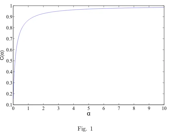
By using MATLAB programme, we can plot the graph ofC(α) as Fig. 1. Here
0 1 2 3 4 5 6 7 8 9 10 0.1
0.2 0.3 0.4 0.5 0.6 0.7 0.8 0.9 1
C(
α
)
α
Fig. 1
From Fig. 1 we see thatC(α) is a strictly increasing function of αwhich can be proved analytically as follows.
Differentiate both sides of (6.2) with respect toµ, we have a linear differential equation ofqλµ(s) =∂qλ(s)/∂µ:
q′
λµ(s) + 2
µqλ(s) + s 1 +s2
qλµ(s) +q2λ(s) = 0, qλ(0) = 0. (6.4)
The solution to (6.4) is
qλµ(s) =−1 +1s2
Z s
0
(1 +τ2) exp
−2µ
Z s
τ
qλ(t) dt
q2λ(τ) dτ <0. (6.5)
While
qλα(s) = ∂qλ(s)
∂µ ∂µ
∂α =qλµ·
−2
α2 >0.
This completes the proof due to (6.3).
7 Appendix
1. The main function routine, MATLAB m-file named bestc.m:
function C=bestc(alpha)
% Input: alpha, may be a scalar or a vector;
% Output: C, the best coefficient corresponding to alpha, When alpha is a vector, C is also a vector with the same size as alpha.
T=.52109530549374738495; % T = sinh(1/2)
G=2.4401300568286909964; % G = T+Tˆ(-1)
options=odeset(’RelTol’,2.221e-14,’ABsTol’,1e-15); % Set ODE solver’s relative error tolerance and absolute error tolerance.
[S,Y]=ode45(@rod,[0,T],0*alpha,options,alpha); % Call ODE solver ode45.
C=Y(end,:)*G;
% End of the main routine.
2. The ODE-file named rod.m is as follows:
function dqds = rod(s,q,alpha)
dqds = (1-2*s*q)/(1+sˆ2)-2*q.ˆ2./alpha;
% End of the ODE-file.
8 Acknowledgment
The authors thank the referee for his/her helpful suggestions. YL is partially supported by NSF of China (Grant No. 10871071 and 10671071). YZ is par-tially supported by Zhejiang Innovation Project (Grant No. T200905), NSF of Zhejiang (Grant No. R6090109) and NSF of China (Grant No. 10971197).
References
[1] Benjamin, T. B.; Bona, J. L.; Mahony, J. J., Model equations for long waves in nonlinear dispersive systems. Philos. Trans. Roy. Soc. London Ser. A 272 (1972), no. 1220, 47–78.
[2] Bressan, A.; Constantin, A., Global conservative solutions of the Camassa-Holm equation. Arch. Rat. Mech. Anal. 183 (2007), 215–239.
[3] Bressan, A.; Constantin, A., Global dissipative solutions of the Camassa-Holm equation, Anal. Appl. 5 (2007), 1–27.
[5] Constantin, A., Existence of permanent and breaking waves for a shal-low water equation: a geometric approach. Ann. Inst. Fourier (Greno-ble) 50 (2000), no. 2, 321–362.
[6] Constantin, A., Finite propagation speed for the Camassa-Holm equa-tion. J. Math. Phys. 46 (2005), 023506, 4pp.
[7] Constantin, A.; Escher, J., Well-posedness, global existence and blow-up phenomena for a periodic quasi-linear hyperbolic equation. Comm. Pure Appl. Math. 51 (1998), 475–504.
[8] Constantin, A.; Escher, J., Wave breaking for nonlinear nonlocal shal-low water equations. Acta Math. 181 (1998), 229–243.
[9] Constantin, A.; Kolev, B., Geodesic flow on the diffeomorphism group of the circle. Comment. Math. Helv. 78 (2003), no. 4, 787–804.
[10] Constantin, A.; Lannes, D., The hydrodynamical relevance of the Camassa-Holm and Degasperis-Procesi equations, Arch. Ration. Mech. Anal. 192 (2009), 165–186.
[11] Constantin, A.; McKean, H. P., A shallow water equation on the circle, Comm. Pure Appl. Math. 52 (1999), 949–982.
[12] Constantin, A.; Molinet, L., Global weak solutions for a shallow water equation. Comm. Math. Phys. 211 (2000), no. 1, 45–61.
[13] Constantin, A.; Strauss, W., Stability of a class of solitary waves in compressible elastic rods. Phys. Lett. A 270 (2000), no. 3–4, 140–148.
[14] Coclite, G. M.; Holden, H.; Karlsen, K. H., Global weak solutions to a generalized hyperelastic-rod wave equation. SIAM J. Math. Anal. 37 (2005), no. 4, 1044–1069.
[15] Coclite, G. M.; Holden, H.; Karlsen, K. H., Wellposedness for a parabolic-elliptic system. Discrete Contin. Dyn. Syst. 13 (2005), no. 3, 659–682.
[16] Dai, H.-H., Model equations for nonlinear dispersive waves in a com-pressible Mooney-Rivlin rod. Acta Mech. 127 (1998), no. 1–4, 193–207.
[17] Dai, H.-H.; Huo, Y., Solitary shock waves and other travelling waves in a general compressible hyperelastic rod. R. Soc. Lond. Proc. Ser. A Math. Phys. Eng. Sci. 456 (2000), no. 1994, 331–363.
[19] Grillakis, M.; Shatah, J.; Strauss, W., Stability theory of solitary waves in the presence of symmetry. I. J. Funct. Anal. 74 (1987), no. 1, 160– 197.
[20] Guo, Z.; Zhou, Y., Wave breaking and persistence properties for the dispersive rod equation. SIAM J. Math. Anal. 40 (2009), no. 6, 2567– 2580.
[21] Himonas, A.; Misio lek, G.; Ponce, G.; Zhou, Y., Persistence Properties and Unique Continuation of solutions of the Camassa-Holm equation. Comm. Math. Phys. 271 (2007), 511–522.
[22] Holden, H.; Raynaud, X., Global conservative solutions of the Camassa-Holm equation–a Lagrangian point of view. Comm. Partial Differential Equations 32 (2007), no. 10–12, 1511–1549.
[23] Holden, H.; Raynaud, X., Global conservative solutions of the gen-eralized hyperelastic-rod wave equation. J. Differential Equations 233 (2007), no. 2, 448–484.
[24] Holden, H.; Raynaud, X., Periodic conservative solutions of the Camassa-Holm equation. Ann. Inst. Fourier (Grenoble) 58 (2008), no. 3, 945–988.
[25] Holden, H.; Raynaud, X., Dissipative solutions for the Camassa-Holm equation. Discrete Contin. Dyn. Syst. 24 (2009), no. 4, 1047–1112.
[26] Ionescu-Kruse, D., Variational derivation of the Camassa-Holm shallow water equation, J. Nonlinear Math. Phys. 14 (2007), 303–312.
[27] Johnson, R. S., Camassa-Holm, Korteweg-de Vries and related models for water waves. J. Fluid Mech. 455 (2002), 63–82.
[28] Kato, T., Quasi-linear equations of evolution, with applications to par-tial differenpar-tial equations. Spectral theory and differenpar-tial equations (Proc. Sympos., Dundee, 1974; dedicated to Konrad Jorgens), pp. 25– 70. Lecture Notes in Math., Vol. 448, Springer, Berlin, 1975.
[29] Kouranbaeva, S., The Camassa-Holm equation as a geodesic ow on the diffeomorphism group, J. Math. Phys. 40 (1999), 857–868.
[30] Li, Y.; Olver, P., Well-posedness and blow-up solutions for an integrable nonlinear dispersive model wave equation. J. Differential Equations 162 (2000), 27–63.
[31] Liu, Y. M.; Zhou, Y., Blow-up phenomenon for a periodic rod equation II. J. Phys. A. 41 (2008), no. 34, 344013, 10 pp.
[33] Molinet, L., On well-posedness results for Camassa-Holm equation on the line: a survey. J. Nonlinear Math. Phys. 11 (2004), no. 4, 521–533.
[34] Seliger, R., A note on the breaking of waves. Proc. Roy. Soc. Lond Ser. A. 303 (1968), 493–496.
[35] Shkoller, S., Geometry and curvature of diffeomorphism groups with
H1 metric and mean hydrodynamics. J. Funct. Anal. 160 (1998), no.
1, 337–365.
[36] Struwe, M., Variational methods. Applications to nonlinear partial dif-ferential equations and Hamiltonian systems. Second edition. Results in Mathematics and Related Areas (3), 34. Springer-Verlag, Berlin, 1996.
[37] Xin, Z.; Zhang, P., On the weak solution to a shallow water equation. Comm. Pure Appl. Math. 53 (2000), 1411–1433.
[38] Zhou, Y., Wave breaking for a periodic shallow water equation. J. Math. Anal. Appl. 290 (2004), 591–604.
[39] Zhou, Y., Wave breaking for a shallow water equation. Nonlinear Anal. 57 (2004), no. 1, 137–152.
[40] Zhou, Y., Stability of solitary waves for a rod equation. Chaos Solitons & Fractals 21 (2004), no. 4, 977–981.
[41] Zhou, Y., Well-posedness and blow-up criteria of solutions for a rod equation. Math. Nachr. 278 (2005), no. 14, 1726–1739.
[42] Zhou, Y., Blow-up phenomenon for a periodic rod equation. Phys. Lett. A 353 (2006), no. 6, 479–486.
[43] Zhou, Y., Blow-up of solutions to a nonlinear dispersive rod equation. Calc. Var. Partial Differential Equations 25 (2006), no. 1, 63–77.
Liangbing Jin
Department of Mathematics Zhejiang Normal University Jinhua, Zhejiang 321004, China
Yongming Liu
Department of Mathematics East China Normal University Shanghai 200241, China [email protected]
Yong Zhou
Department of Mathematics Zhejiang Normal University Jinhua, Zhejiang 321004, China