LINEAR ALGEBRA AND THE SUMS OF POWERS OF INTEGERS∗
FRANC¸ OIS DUBEAU†
Abstract. A general framework based on linear algebra is presented to obtain old and new polynomial expressions for the sums of powers of integers. This framework uses changes of polynomial basis, infinite lower triangular matrices and finite differences.
Key words. Finite differences, Polynomial space, Polynomial basis, Change of basis, Sum of powers of integers, Infinite lower triangular matrix.
AMS subject classifications.11B83, 11B37, 15A03, 15A09.
1. Introduction. Polynomial formulas to evaluate the sums of powers of inte-gers
K
k=1
kn= 1n+ 2n+ 3n+· · ·+Kn
has a long history. In the antic Greece, Archimedes (287BC−212BC) obtained expressions for n = 1 and n = 2, andduring the apex of Arab mathematical sci-ence, in the eleven century, Al-Haytham (965-1038), known in the West has Alhazen, obtainedformulas for n= 3 andn= 4 [4, 8]. Later several mathematicians consid-eredthis problem: Faulhaber (1631), Pascal (1636), Fermat (1654), Bernoulli (1713), Euler (1755), Jacobi (1824), etc. The most celebratedresults were obtainedby J. Faulhaber [10, 12, 20, 7, 14, 13] andJ. Bernoulli [19, 14]. The reader interestedby the history of this problem couldlook at the preceding references andthe following [2, 6, 9, 15, 18, 19, 21].
In this paper we present a unifiedapproach for obtaining polynomial formulas for the sums of powers of integers. The methodis basedon finite differences andchanges of basis for polynomial subspaces. The main result is the following theorem proved in Section 2.
Theorem 1.1. Let Bp =pi(x)+∞
i=0 be any family of polynomials such that the
∗Received by the editors August 6, 2008. Accepted for publication November 16, 2008. Handling
Editor: Miroslav Fiedler.
†D´epartement de math´ematiques, Facult´e des sciences, Universit´e de Sherbrooke, 2500 Boul. de
l’Universit´e, Sherbrooke (Qc), Canada, J1K 2R1 ([email protected]). Supported by an NSERC (Natural Sciences and Engineering Research Council of Canada) individual discovery grant.
polynomial pi(x) is of degree i. For any fixed real number τ and any integer n≥0
there exist constants αn,j(τ)
n
j=−1 such that
K
k=1
kn=
n
j=−1
αn,j(τ)pj+1(K+τ)
(1.1)
where
αn,−1(τ) =−
n
j=0
αn,j(τ)pj+1(τ) =−
n
j=0
αn,j(τ)pj+1(τ−1).
(1.2)
Well known examples of formulas that we can obtain from this result are the Bernoulli’s polynomial expression [19, 14] (see Section 3), andthe Faulhaber’s poly-nomial expressions [10] (see Section 4.3).
In the last section the methodis extendedto obtain polynomial expressions for thel-fold
Σ(Kl)0K1n =
K1
kl=K0
kl
kl−1=K0
· · ·
k3
k2=K0
k2
k1=K0
k1n
l summations
(1.3)
Finally, let us observe that the methodworkedout in this paper is also suitable for implementation in a computer algebra system.
2. A general method for Kk=1kn. LetB
p=pi(x)+
∞
i=0 be a family of
poly-nomials wherepi(x) is of d egreei fori≥0. Let ∆τ be the finite difference operator
defined for any fixedτ∈Randfor any functionF(x) by
∆τF(x) =F(x+τ)−F(x+τ−1).
The methodis basedon the following two elementary results.
Lemma 2.1. For any integerK0≤K1 we have
K1
k=K0
∆τF(x+k) =F(x+K1+τ)−F(x+K0+τ−1).
(2.1)
Lemma 2.2. For any integer i ≥ 0, if pi(x) is a polynomial of degree i, then
As a consequence of Lemma 2.2, for any integern ≥0 the sets Bn
s =
ei(x) =
xini=0, and Bn
q =
qi(x) = ∆τpi+1(x) n
i=0 are bases for the setPn of polynomials of
degree at mostn, and
Pn= Lin
ei(x)|i= 0, ..., n
= Linqi(x)|i= 0, ..., n
.
(2.2)
Let −→E(x) = (e0(x), e1(x), e2(x),· · ·)t and −→Q(x) = (q0(x), q1(x), q2(x),· · ·)t then
from (2.2) we obtain
− →
E(x) =M−→Q(x) and −→Q(x) =N−→E(x) (2.3)
whereM andN are two infinite lower triangular matrices given by
M = αi,j(τ)
i= 0,1, ... j= 0,1, ...
=
α0,0(τ) 0 · · · α1,0(τ) α1,1(τ) 0 · · · α2,0(τ) α2,1(τ) α2,2(τ) 0 · · ·
..
. ... ... . .. ...
and
N = βi,j(τ)
i= 0,1, ... j= 0,1, ...
=
β0,0(τ) 0 · · · β1,0(τ) β1,1(τ) 0 · · · β2,0(τ) β2,1(τ) β2,2(τ) 0 · · ·
..
. ... ... . .. ...
.
These matrices are invertible andM N =I=N M.
From (2.3) and(2.1), we obtain
K1
k=K0
en(x+k) = n
j=0 αn,j(τ)
pj+1(x+K1+τ)−pj+1(x+K0+τ−1)
,
(2.4)
andif we set x = 0, K0 ≤ K1 = K, and K0 = 0 or 1, then we have a proof of Theorem 1.1.
We suggest two methods for computing the scalarsαi,j(τ)’s. The first methodis
by direct inversion of the infinite lower triangular matrixN while the secondmethod uses the derivative ofqn(x).
For the first method, we consider the systemM N=I andwe obtain
αi,j(τ) =
1
βi,i(τ) for j=i,
or we consider the systemN M =Iandwe have
αi,j(τ) =
− 1
βi,i(τ)
i−1
l=jβi,l(τ)αl,j(τ) for j= 0, ..., i−1,
1
βi,i(τ) for j=i.
The secondmethodproceeds as follows. Sincep(1)n+1(x) is a polynomial of degree
n, we can write
p(1)n+1(x) =
n
j=0
γn,j−1pj(x),
and
qn(1)(x) = ∆τp(1)n+1(x) =
n
j=1
γn,j−1∆τpj(x) = n−1
j=0
γn,jqj(x).
Using the matrix notation, we have
− →
Q(1)(x) = Γ−→Q(x) (2.5)
where Γ is the infinite lower triangular matrix
Γ = γi,j
i= 0,1, ... j= 0,1, ...
=
0 · · · γ1,0 0 · · · γ2,0 γ2,1 0 · · · γ3,0 γ3,1 γ3,2 0 · · ·
..
. ... ... . .. ...
.
Moreover, we also have
− →
E(1)(x) =DP−→E(x),
(2.6)
where the infinite diagonal matricesD andP are defined by
D=
0 0
0 1 0
0 2 0
0 3 0
. .. ... ...
and P=
0 1 0
0 1 0
0 1 0
. .. ... ...
.
We obtain recursively each line ofM by solving the system
DP M=MΓ, −
→
E(ξ) =M−→Q(ξ),
where ξ is any arbitrary value for x. This lead s to : α0,0(τ) = 0, and for i≥ 1 we
have
αi,j(τ) =
i
γ i,i−1αi−1,i−1(τ) for j=i,
1
γ j,j−1
iαi−1,j(τ)−il=j+1αi,l(τ)γl,j−1
for j=i−1, ...,1,
ei(ξ)− P
i
j=1αi,j(τ)qj(ξ)
q0(ξ) for j= 0.
3. Bernoulli’s polynomial formula. LetBp=pi(x) =ei(x)+ ∞
i=0 andτ= 0.
We will use the notationαi,j(τ) =αi,j andβi,j(τ) =βi,j. We have
qn(x) =en+1(x)−en+1(x−1) =
n
j=0
n+ 1
j
(−1)n−jej(x),
(3.1)
henceβn,j=
n+ 1
j
(−1)n−j forj= 0, ..., n, and
N =
1 0 · · · −1 2 0 · · ·
1 −3 3 0 · · · −1 4 −6 4 0 · · ·
..
. ... ... ... . .. ...
.
To compute M we use (2.5), andsince qn(1)(x) = (n+ 1)qn−1(x) for n ≥1, we
have
Γ =
0
2 0
0 3 0
0 4 0
. .. ... ...
= (I+D)P.
Then solving the system
DP M =M(I+D)P, −
→
leads to : α0,0= 1, and for i≥1
αi,j=
i
j+ 1αi−1,j−1
forj= 1, ..., i, and
αi,0=
i
j=1
(−1)j+1αi,j= 1− i
j=1
αi,j.
(3.2)
From these relations we obtain
αi,j = 1
i+ 1
i+ 1
j+ 1
αi−j,0
(3.3)
forj= 0, ..., i.
Remark 3.1. From (3.2) and(3.3), if we set αi−j,0 = Bi, the Bi’s are the
Bernoulli’s numbers generatedby : B0= 1, and fori≥1
i
j=0
(−1)j
i+ 1
j+ 1
Bi−j= 0 or 1
i+ 1
i
j=0
i+ 1
j+ 1
Bi−j = 1.
(3.4)
Fori≥1, from (3.4) we get
2
i+ 1 ⌊i
2⌋
j=0
i+ 1
2j
B2j= 1,
(3.5)
and
2
i+ 1 ⌊i−1
2 ⌋
j=0
i+ 1 2j+ 1
B2j+1= 1.
(3.6)
SinceB0= 1, from (3.5) we obtain theB2j’s forj ≥1. From (3.6) we haveB1= 12
andfori≥3
⌊i−1 2 ⌋
j=1
i+ 1 2j+ 1
B2j+1= 0,
which implies thatB2j+1= 0 forj≥1.
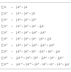
In this case (1.1) leads to the following celebrated Bernoulli’s polynomial formula
K
k=1
kn= 1
n+ 1
n
i=0
n+ 1
i
BiKn+1−i.
K = 12K2+12K
K2 = 1
3K 3+1
2K 2+1
6K
K3 = 1
4K 4+1
2K 3+1
4K 2
K4 = 1
5K5+ 1 2K4+
1 3K3−
1 30K
K5 = 1
6K 6+1
2K 5+ 5
12K 4− 1
12K 2
K6 = 1
7K7+ 1 2K6+
1 2K5−
1 6K3+
1 42K
K7 = 1
8K 8+1
2K 7+ 7
12K 6− 7
24K 4+ 1
12K 2
K8 = 1
9K9+ 1 2K8+
2 3K7−
7 15K5+
2 9K3−
1 30K
K9 = 1
10K 10+1
2K 9+3
4K 8− 7
10K 6+1
2K 4− 3
20K 2
K10 = 1 11K11+
1 2K10+
5
6K9−1K7+ 1K5− 1 2K3+
[image:7.612.110.405.93.392.2]5 66K
Table 3.1
First10Bernoulli’s polynomial expressions for the sums of powers of integers.
4. Towards the Faulhaber’s polynomial formula. In this section we present three formulas for the sums of powers of integers relatedby the bases we use to obtain them. The last one is the Faulhaber’s polynomial formula. Throughout this section
τ= 12.
4.1. A first intermediate polynomial formula. The first formula of this section is very similar to the Bernoulli’s polynomial formula. Let Bp = pi(x) =
ei(x)+ ∞
i=0, andlet us use the notationui(x) = ∆1/2pi+1(x),ai,j =αi,j( 1
2) andbi,j= βi,j(12).
N1−→E(x) where
M1= ai,j
i= 0,1, ... j= 0,1, ...
=
a0,0 0 · · · a1,0 a1,1 0 · · · a2,0 a2,1 a2,2 0 · · ·
.. . ... ... . .. ... and
N1= bi,j
i= 0,1, ... j= 0,1, ...
=
b0,0 0 · · · b1,0 b1,1 0 · · · b2,0 b2,1 b2,2 0 · · ·
.. . ... ... . .. ... . We have
un(x) =en+1(x+
1
2)−en+1(x− 1 2) = n j=0
n+ 1
j
(1 2)
n+1−j[1 + (−1)n−j]e j(x),
= ⌊n 2⌋ j=0
n+ 1 2j+ 1
(1 2)
2je
n−2j(x),
(4.1) andhence N1=
1 0 · · ·
0
2 1
0 · · ·
1 22 3 3 0 3 1
0 · · ·
0 212
4 3 0 4 1
0 · · ·
1 24 5 5 0 1 22 5 3 0 5 1
0 · · ·
.. . ... ... ... . .. . .. ... .
From (4.1), we not only have (2.2) but also
Lin{en−2i(x)|i= 0, ...,⌊
n
2⌋}= Lin{un−2i(x)|i= 0, ...,⌊
n
andthis observation implies that an,n−(2j+1) = 0 =bn,n−(2j+1) forj = 0, ...,⌊n−21⌋.
Therefore the sum of powers of integers (1.1) is given by
K
k=1
kn=an,−1+
⌊n
2⌋
j=0
an,n−2j(K+1
2)
n+1−2j
(4.2)
with (1.2) as
an,−1=−
⌊n
2⌋
j=0
(1 2)
n+1−2ja
n,n−2j= (−1)n
⌊n
2⌋
j=0
(1 2)
n+1−2ja n,n−2j.
(4.3)
It follows thatan,−1= 0 forneven.
Using (2.5), andsinceqn(1)(x) = (n+ 1)qn−1(x) forn≥1, we have
Γ = (I+D)P =
0
2 0
0 3 0
0 4 0
. .. ... ...
.
Solving the system
DP M1=M1(I+D)P, −
→
E(0) =M1−→U(0) or →−E(1) =M1−→U(1),
leads to : a0,0= 1, and fori≥1
ai,j=
i
j+ 1ai−1,j−1
forj= 1, ..., i, and
ai,0=−
i
j=1
(1 2)
j+1[1 + (−1)j]a
i,j=−[1 + (−1) i]
2
i−1 2
j=0
(1 2)
i−2ja i,i−2j.
(4.4)
Henceai,0= 0 for od d i. From these relations we obtain
ai,j =
1
i+ 1
i+ 1
j+ 1
ai−j,0
(4.5)
Remark 4.1. As for the Bernoulli’s numbers, let us set ai,0 =Ai. Then from
(4.4) and(4.5), theAi’s are generatedby : A0= 1 and fori≥1
i
2
j=0
(1 2)
2j
i+ 1 2j+ 1
Ai−2j = 0.
Usingx=1
2 andx=− 1 2 in
− →
E(x) =M1−→U(x) , we have
1 2
i
=
i
j=0
ai,j and −1
2
i
=
i
j=0
(−1)jai,j
which leads to
1 2
i
= ⌊i
2⌋
j=0
ai,i−2j and0 = ⌊i−1
2 ⌋
j=0
ai,i−(2j+1).
We also conclude from these relations that ai,i−(2j+1) = 0 and A2j+1 = 0 for any j≥0.
Finally, (4.2) becomes
K
k=1
kn= ⌊n+1
2 ⌋
j=0
an,n−2j(K+1
2)
n+1−2j.
where thean,n−2j’s are given by (4.3), (4.4) and(4.5).
4.2. A second intermediate polynomial formula. Let Bp = pi(x)+ ∞ i=0
where
pi(x) =
ei(x) for i= 0,1,
ei(x)−14ei−2(x) for i≥2.
Let us use the notationvi(x) = ∆1/2pi+1(x),ci,j=αi,j(12) anddi,j=βi,j(12).
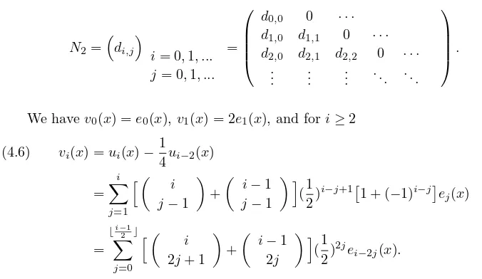
Let −→V(x) = (v0(x), v1(x), v2(x),· · ·)t, and set −→E(x) = M2→−V(x) and −→V(x) =
N2−→E(x) where the two lower triangular matrices are defined by
M2= ci,j
i= 0,1, ... j= 0,1, ...
=
c0,0 0 · · · c1,0 c1,1 0 · · · c2,0 c2,1 c2,2 0 · · ·
..
. ... ... . .. ...
K = 12U2−18
K2 = 1
3U 3− 1
12U
K3 = 1
4U 4−1
8U 2+ 1
64
K4 = 1
5U5− 1 6U3+
7 240U
K5 = 1
6U 6− 5
24U 4+ 7
96U 2− 1
128
K6 = 1
7U7− 1 4U5+
7 48U3−
31 1344U
K7 = 1
8U 8− 7
24U 6+ 49
192U 4− 31
384U 2+ 17
2048
K8 = 1
9U9− 1 3U7+
49 120U5−
31 144U3+
127 3840U
K9 = 1
10U 10−3
8U 8+49
80U 6−31
64U 4+ 381
2560U 2− 31
2048
K10 = 1 11U11−
5 12U9+
7 8U7−
31 32U5+
127 256U3−
[image:11.612.71.409.454.650.2]2555 33792U
Table 4.1
First10Bernoulli’s like polynomial expressions for the sums of powers of integers,U=K+1
2.
and
N2= di,j
i= 0,1, ... j= 0,1, ...
=
d0,0 0 · · · d1,0 d1,1 0 · · · d2,0 d2,1 d2,2 0 · · ·
.. . ... ... . .. ... .
We havev0(x) =e0(x),v1(x) = 2e1(x), andfori≥2
vi(x) =ui(x)−
1
4ui−2(x) (4.6) = i j=1 i j−1
+
i−1
j−1 ( 1 2)
i−j+11 + (−1)i−je j(x)
= ⌊i−1
2 ⌋
j=0
i
2j+ 1
+
i−1
2j (
1 2)
Hence
N2=
1 0 · · ·
0 2 0 · · ·
0 0 3 0 · · ·
0 12 0 4 0 · · ·
0 0 7
4 0 5 0 · · ·
0 18 0 4 0 6 0 · · ·
..
. . .. ... ... ... ... ...
.
Then forn≥1
Lin{en−2i(x)|i= 0, ...,⌊
n−1
2 ⌋}= Lin{vn−2i(x)|i= 0, ...,⌊
n−1 2 ⌋},
and cn,0 = 0 =dn,0 for n≥1, and cn,n−(2j+1) = 0 =dn,n−(2j+1)cn,n−(2j+1) = 0 = dn,n−(2j+1)for anyj= 0, ...,⌊n−21⌋. It follows that (1.1) becomes
K
k=1
kn=
K(K+ 1)n−
1 2
j=0 cn,n−2j(K+21)n−1−2j fornodd,
K(K+ 1)(K+1 2)
n
2−1
j=0 cn,n−2j(K+21)n−2−2j forneven.
Remark 4.2. From (4.6) we have −→V(x) = (I − 14P2)−→U(x). Then −→E(x) = M2(I−1
4P
2)−→U(x). We also have−→E(x) =M1−→U(x). It follows thatM2(I−1 4P
2) =M1.
But (I− 1 4P
2)−1 = +∞ l=0(14)
lP2l, then M2 =M1(I−1 4P
2)−1 =M1+∞ l=0(14)
lP2l,
and
ci,i−2j = j
l=0
(1 4)
j−la i,i−2l
forj= 0, ...,⌊i
2⌋.
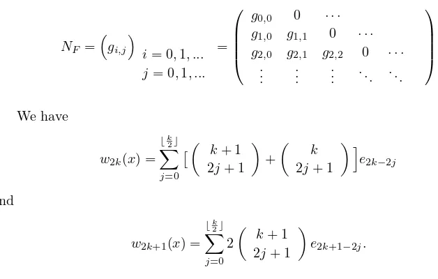
4.3. Faulhaber’s polynomial formula. LetBp=pi(x)+ ∞ i=0 where
pi(x) =xi−2⌊
i
2⌋(x−1
2)(x+ 1 2)
⌊i
2⌋.
Let us use the notationwi(x) = ∆1/2pi+1(x),fi,j=αi,j(12), andgi,j=βi,j(12).
Let −W→(x) = (w0(x), w1(x), w2(x),· · ·)t, then −→E(x) = M
F−W→(x) and −W→(x) =
NF−→E(x) where the two lower triangular matrices are defined by
MF = fi,j
i= 0,1, ... j = 0,1, ...
=
f0,0 0 · · · f1,0 f1,1 0 · · · f2,0 f2,1 f2,2 0 · · ·
..
. ... ... . .. ...
K = 12V
K2 = 1
3U V
K3 = V[1 4U
2− 1 16]
K4 = U V[1 5U2−
7 60]
K5 = V[1 6U
4−1 6U
2+ 1 32]
K6 = U V[1 7U4−
3 14U2+
31 336]
K7 = V[1 8U
6−25 96U
4+ 73 384U
2− 17 512]
K8 = U V[1 9U6−
11 36U4+
239 720U2−
127 960]
K9 = V[1 10U
8− 7 20U
6+21 40U
4−113 320U
2+ 31 512]
K10 = U V[1 11U8−
13 33U6+
205 264U4−
409 528U2+
[image:13.612.78.392.455.655.2]2555 8448]
Table 4.2
First10intermediate polynomial expressions for the sums of powers of integers,V =K(K+ 1).
and
NF = gi,j
i= 0,1, ... j = 0,1, ...
=
g0,0 0 · · · g1,0 g1,1 0 · · · g2,0 g2,1 g2,2 0 · · ·
..
. ... ... . .. ...
We have
w2k(x) = ⌊k
2⌋
j=0
k+ 1
2j+ 1
+
k
2j+ 1 e2k−2j
and
w2k+1(x) =
⌊k
2⌋
j=0
2
k+ 1 2j+ 1
The matrixNF is
NF =
1 0 · · ·
0 2 0 · · ·
0 0 3 0 · · ·
0 0 0 4 0 · · ·
0 0 1 0 5 0 · · ·
0 0 0 2 0 6 0 · · ·
..
. ... ... ... ... ... . .. ...
.
Consequently fori≥2
Linwi−2j(x)|j= 0, ...,⌊
i
2⌋ −1
= Linei−2j(x)|j = 0, ...,⌊
i
2⌋ −1
,
andalso
ei(x) = ⌊i
2⌋−1
j=0
fi,i−2jwi−2j(x).
(4.7)
Hence, forn≥2, (1.1) becomes
K
k=1
kn=
K(K+ 1)2 n−3
2
j=0 fn,n−2jK(K+ 1)
n−3 2 −j
fornodd,
(K+12)K(K+ 1)n2−1
j=0 fn,n−2jK(K+ 1)
n
2−1−j forneven,
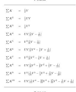
which is the Faulhaber’s polynomial expression for the sums of powers of integers.
To compute recursively the coefficientsfi,i−2j, we observe that
w2(1)l+2(x) = (1 + 2(l+ 1))w2l+1(x) + l+ 1
2 w2l−1(x), (4.8)
and
w2(1)l+1(x) = 2(l+ 1)w2l(x).
(4.9)
Then, from (4.7)
(2l+ 2)x2l+1=
l
j=0
f2l+2,2l+2−2j
(1 + 2(l−j+ 1))w2(l−j)+1(x)
(4.10)
+(l−j) + 1
2 w2(l−j)−1(x)
,
(4.11)
and
(2l+ 1)x2l=
l−1
j=0
f2l+1,2l+1−2j2(l−j+ 1))w2(l−j)(x).
Then again using (4.7), (4.8) and(4.9), we obtain the recursive method: assume
f2,0= 0 andf2,2=13, forl≥1 :
(a) to computef2l+1,2l+1−2j from f2l,2l−2j we use the relation
f2l+1,2l+1−2j=
(2l+ 1)
2(l+ 1−j)f2l,2l−2j (4.13)
forj= 0, ..., l−1;
(b) to computef2l+2,2l+2−2j fromf2l+1,2l+1−2j, we setf2l+2,2l+4= 0 andf2l+1,1= 0
andwe use
f2l+2,2l+2−2j=
2(l+ 1) (2(l−j) + 3)
f2l+1,2l+1−2j−
(l+ 2−j)
4(l+ 1) f2l+2,2l+2−2(j−1)
(4.14)
forj= 0, ..., l.
Remark 4.3. Using the matrix notation, (4.8) and(4.9) leadto the lower
trian-gular matrix Γ such that−W→(1)(x) = ΓW−→(x) andits nonzero elements areγi,i−1=i+1
fori≥1, and γ2l,2l−3= 4l forl≥2. Solving the systemDP MF =MFΓ, we obtain
(4.13) and(4.14).
The formula (4.13) was known by Faulhaber [10, 14] andappears also in [12, 20, 7, 15].
4.4. Other polynomial formulas. We couldfindother formulas trying with other setsB. For example, take any integerm≥2 and setpi(x) =ei(x) fori≤0 and
pi(x) =xi−2⌊
i m⌋
(x−1
2)(x+ 1 2)
⌊i m⌋
fori≥1. The valuem= 2 corresponds to the Faulhaber’s case.
5. An extension of the method. In this section by repeating the application of the difference operator we obtain expressions for l-foldsummations of powers of integers. Let us use the following notation for thel-foldsummations
Σ(Kl)0∆
σ
τF(x+K1) =
∆σ
τF(x+K1) for l= 0,
ΣK1
kl=K0· · ·Σ
k2
k1=K0∆
σ
τF(x+k1) for l≥1,
and
Σ(Kl)0K10=
1 for l= 0,
ΣK1
kl=K0· · ·Σ
k2
k1=K01 for l≥1,
K = 12V
K2 = 1
3U V
K3 = 1
4V 2
K4 = U V[1 5V −
1 15]
K5 = V2[1 6V −
1 12]
K6 = U V[1 7V2−
1 7V +
1 21]
K7 = V2[1 8V
2−1 6V +
1 12]
K8 = U V[1 9V3−
2 9V2+
1 5V −
1 15]
K9 = V2[1 10V
3−1 4V
2+ 3 10V −
3 20]
K10 = U V[1 11V4−
10 33V3+
17 33V2−
5 11V +
[image:16.612.122.378.87.396.2]5 33]
Table 4.3
First10Faulhaber’s polynomial expressions for the sums of powers of integers.
Lemma 5.1. For any integersK0≤K1 andσ≥1 we have
ΣK1
k=K0∆
σ
τF(x+k) = ∆τσ−1F(x+K1+τ)−∆στ−1F(x+K0+τ−1).
More generally we have
Lemma 5.2. For any integersK0≤K1 and0≤l≤σ we have
Σ(Kl)0∆στF(x+K1) = ∆στ−lF(x+K1+lτ)
−Σlj−=01
ΣK(j)0K10∆τσ−(l−j)F(x+K0+ (l−j)τ−1).
Lemma 5.3. For any integer i ≥ 0, if pi(x) is a polynomial of degree i, then
qi(x) = ∆στpi+σ(x) is a polynomial of degreei.
From Lemma 5.3 we have
Pn= Lin
ei(x)|i= 0, ..., n
= Linqi(x)|i= 0, ..., n
Let−→E(x) = M−→Q(x) and →−Q(x) =N−→E(x) whereM andN are two lower triangular matrices
M = αi,j(τ, σ)
i= 0,1, ... j= 0,1, ...
=
α0,0(τ, σ) 0 · · ·
α1,0(τ, σ) α1,1(τ, σ) 0 · · · α2,0(τ, σ) α2,1(τ, σ) α2,2(τ, σ) 0 · · ·
..
. ... ... . .. ...
and
N = βi,j(τ, σ)
i= 0,1, ... j= 0,1, ...
=
β0,0(τ, σ)) 0 · · ·
β1,0(τ, σ)) β1,1(τ, σ)) 0 · · · β2,0(τ, σ)) β2,1(τ, σ)) β2,2(τ, σ)) 0 · · ·
..
. ... ... . .. ...
,
such thatM N =I=N M. It follows that
ei(x) = i
j=0
αi,j(τ, σ)qj(x) = i
j=0
αi,j(τ, σ)∆στpj+σ(x),
(5.1)
and
qi(x) = i
j=0
βi,j(τ, σ)ej(x).
From (5.1) andthe Lemma 5.2 we have
Σ(Kl)0(x+K1)n=
n
j=0
αn,j(τ, σ)Σ(Kl)0∆
σ
τpj+σ(x+K1).
If we setx= 0 and 1 =K0≤K1=K, thel-foldsummation of powers of integers is
Σ(1l)Kn =
n
j=0
αn,j(τ, σ)Σ(1l)∆
σ
τpj+σ(K).
The scalars αi,j(τ, σ)’s can be computedrecursively by inversion of the lower
p(1)n+σ(x) is a polynomial of degree n+σ−1, we have
p(1)n+σ(x) =
n+σ−1
j=0
γn,j−σpj(x).
Then
qn(1)(x) = ∆στp
(1)
n+σ(x) = n+σ−1
j=σ
γn,j−σ∆στpj(x) = n−1
j=0
γn,jqj(x),
andwe write−→Q(1)(x) = Γ−→Q(x) where Γ is a lower triangular matrix with zero values on the diagonal. We also have −→E(1)(x) = DP−→E(x). Using these identities with
− →
E(1)(x) =M−→Q(1)(x), it follows that
DP M =MΓ.
Adding
− →
E(ξ) =M−→Q(ξ)
for any fixedx=ξ, we can solve forM.
6. Examples. We present two families of formulas basedon the general ap-proach. The details are left to the reader.
6.1. A Bernoulli’s type example. Let Bp =
pi(x) = ei(x)
+∞
i=0, and let us
use the notation ui(x) = ∆σ1/2pi+σ(x), ai,j(σ) = αi,j(12, σ) and bi,j(σ) = βi,j(12, σ). We
have
un(x) = ⌊n
2⌋
j=0
b(n,nσ)−2jen−2j(x)
then
Lin{en−2i(x)|i= 0, ...,⌊
n
2⌋}= Lin{un−2i(x)|i= 0, ...,⌊
n
2⌋}. It follows that
en(x) = ⌊n
2⌋
j=0
a(n,nσ)−2jun−2j(x) = ⌊n
2⌋
j=0
a(n,nσ)−2j∆σ
1/2pn+σ−2j(x).
and
Σ(1σ)Kn=
⌊n
2⌋
j=0
For example, letσ= 2 we have
Σ(2)1 Kn =
⌊n
2⌋
j=0
a(2)n,n−2j(K+ 1)n+2−2j−(K+ 1).
6.2. A Faulhaber’s type example. LetBp=pi(x)+ ∞
i=0 with
pi(x) =xi−2⌊
i
2⌋(x−σ1
2)(x+σ 1 2)
⌊i
2⌋
for i≥1. We use the notation wi(x) = ∆σ1/2pi+σ(x), fi,j(σ) =αi,j(12, σ), and g(i,jσ) =
βi,j(12, σ). It is possible to show that
wi(x) = ⌊i−1
2 ⌋
j=0
g(i,iσ)−2jei−2j(x)
withgi,(σ0)= 0 and fi,(σ0)= 0. Then
Linei−2j(x)|j= 0, ...,⌊
i−1 2 ⌋
= Linwi−2j(x)|j = 0, ...,⌊
i−1 2 ⌋
,
and we can write
en(x) = ⌊n−1
2 ⌋
j=0
fn,n(σ)−2jwn−2j(x) = ⌊n−1
2 ⌋
j=0
fn,n(σ)−2j∆σ1/2pn+σ−2j(x)
andobtain
Σ(1σ)Kn = ⌊n−1
2 ⌋
j=0
fn,n(σ)−2jΣ(1σ)∆σ1/2pn+σ−2j(K).
For example, forσ= 2 we have
Σ(2)1 Kn =
⌊n−1 2 ⌋
j=0
fn,n(2)−2jΣ(2)1 ∆12/2pn+2−2j(K)
= ⌊n−1
2 ⌋
j=0
fn,n(2)−2j(K+ 1)n−2⌊n2⌋
K(K+ 2)⌊ n
2⌋+1−j
REFERENCES
[1] D. Acu. Some algorithms for the sums of integer powers.Mathematics Magazine, 61:189–191, 1988.
[2] A. F. Beardon. Sums of powers of integers. American Mathematical Monthly, 103:201–213, 1996.
[3] D. M. Bloom. An old algorithm for the sums of integer powers. Mathematics Magazine, 66:304–305, 1993.
[4] C. B. Boyer. Pascal’s formula for the sums of powers of integers. Scripta Mathematica, 9: 237-244, 1943.
[5] M. A. Budin and A. J. Cantor. Simplified computation of sums of powers of integers. IEEE Transactions on Systems, Man, and Cybernetics, 2:285–286, 1972.
[6] A. W. F. Edwards. Sums of powers of integers : a little of history. The Mathematical Gazette, 66:22–28, 1982.
[7] A. W. F. Edwards. A quick route to sums of powers.American Mathematical Monthly, 93:451– 455, 1986.
[8] C. H. Jr Edwards. The Historical Development of Calculus. Springer-Verlag Inc., New York, 1979.
[9] H. M. Edwards.Fermat’s Last Theorem : a Genetic Introduction to Algebraic Number Theory. Springer-Verlag Inc. New York, New York, 1977.
[10] J. Faulhaber. Academia Algebræ. Darinnen die miraculosische Inventiones zu den h¨ochsten weiterscontinuirtundprofitiertwerden, call number QA154.8 F3 1631a f MATH at Stan-ford University Libraries, Johann Ulrich Sch¨onigs, Augspurg[sic], 1631.
[11] G. H. Hardy and E. M. Wright. An Introduction to the Theory of Numbers. 4th edition, Oxford, London, 1960.
[12] J. Jacobi. De usu legitimo formulae summatoriae Maclaurinianae. Journal f¨ur die Reine und Angewandte Mathematik, 12:263-272, 1834.
[13] H. K. Krishnapriyan. Eulerian polynomial and Faulhaber’s result on sums of powers of integers.
The College Mathematics Journal, 26:118-123, 1995.
[14] D. E. Knuth. Johann Faulhaber and sums of powers. Mathematics of Computation, 203:277– 294, 1993.
[15] T. C. T. Kotiah. Sums of powers of integers - A review.International Journal of Mathematical Education in Science and Technology, 24:863–874, 1993.
[16] J. Nunemacher and R. M. Young. On the sum of consecutive Kth powers. Mathematics
Magazine, 61:237–238, 1987.
[17] R. W. Owens. Sums of powers of integers. Mathematics Magazine, 65:38–40, 1992.
[18] S. H. Scott. Sums of powers of natural numbers by coefficient operation. The Mathematical Gazette, 64:231–238, 1980.
[19] D. E. Smith. A Source Book in Mathematics. McGraw-Hill, New York, 1929. [20] L. Tits. Sur la sommation des puissances num´eriques. Mathesis, 37:353-355, 1923.