A Lax Formalism for the Elliptic Dif ference
Painlev´
e Equation
⋆Yasuhiko YAMADA
Department of Mathematics, Faculty of Science, Kobe University, Hyogo 657-8501, Japan
E-mail: [email protected]
Received November 20, 2008, in final form March 25, 2009; Published online April 08, 2009 doi:10.3842/SIGMA.2009.042
Abstract. A Lax formalism for the elliptic Painlev´e equation is presented. The construction is based on the geometry of the curves on P1 ×P1 and described in terms of the point configurations.
Key words: elliptic Painlev´e equation; Lax formalism; algebraic curves
2000 Mathematics Subject Classification: 34A05; 14E07; 14H52
1
Introduction
The difference analogs of the Painlev´e differential equations have been extensively studied in the last two decades (see [6, 12] for example). It is now widely recognized that some of the aspects of the Painlev´e equations, in particular their algebraic or geometric properties, can be understood in universal way by considering differential and difference cases together.
In [12], Sakai studied the difference Painlev´e equations from the point of view of rational surfaces and classified them into three categories: additive, multiplicative (q-difference) and elliptic1. The classification is summarized in the following diagram:
ell. E8(1)
Z
ր
mul. E8(1)→E7(1)→E6(1)→D(1)5 →A(1)4 →(A2+A1)(1)→(A1+A1)(1)→A(1)1 → D6
add. E8(1)→E7(1)→E6(1) → D4(1)→ A(1)3 →(A1+A1)(1)→A(1)1 →Z2
ց ց ↓
A(1)2 →A(1)1 → 1
Among them, Sakai’s elliptic Painlev´e equation [12] is the master equation of all the second order Painlev´e equations. It has the affine Weyl group symmetry of typeE(1)8 and all the other cases arise as its degenerations.
It is well known that the differential Painlev´e equations describe iso-monodromy deformations of linear differential equations. Since the iso-monodromy interpretation of the Painlev´e equations is a main source of variety of deep properties of the latter, it is an important problem to find Lax formalisms for difference cases.
⋆This paper is a contribution to the Proceedings of the Workshop “Elliptic Integrable Systems, Isomonodromy
Problems, and Hypergeometric Functions” (July 21–25, 2008, MPIM, Bonn, Germany). The full collection is available athttp://www.emis.de/journals/SIGMA/Elliptic-Integrable-Systems.html
1
In fact, for some of difference Painlev´e equations, the Lax formulations have been known (see [1, 3, 4, 5, 7] for example). Let us give an example of q-difference case with symmetry of type D5(1). The equation is Jimbo–Sakai’s q-PVI equation [7] which is a discrete dynamical system defined by the following birational transformation:
T :
The q-PVI equation (1) was originally derived as the compatibility of certain 2×2 matrix Lax pair:
Y(qz) =A(z)Y(z), T(Y(z)) =B(z)Y(z),
which is equivalent (up to a gauge transformation) with the following scalar Lax pair for the first componenty of Y. One of the scalar Lax equations is
(a1−z)(a2−z) In elliptic case, it is natural to expect a scalar Lax pair which looks like
C1y(z−δ) +C2y(z) +C3y(z+δ) = 0, C4y(z−δ) +C5y(z) +C6T(y(z)) = 0, (4) where the coefficients C1, . . . , C6 are elliptic functions on variables z and other parameters. However, the explicit construction of such Lax formalism has remained as a difficult problem because of the complicated elliptic dependence including many parameters.
In this paper, we give a Lax formulation for the elliptic Painlev´e equation withE8(1) symmetry using a geometric method. The main idea is to consider the Lax pair (4) as equations for algebraic curves with respect to the unknown variables of the Painlev´e equation. We note that the Lax pair for the additive difference E8(1) case was obtained by Boalch [4]. For the elliptic case, another approach has recently proposed by Arinkin, Borodin and Rains [2,11].
This paper is organised as follows. In Section2, a geometric description of the elliptic Painlev´e equation is reviewed in P1 ×P1 formalism. In Section 3 the Lax pair for the elliptic Painlev´e
equation is formulated. Some properties of relevant polynomials are prepared in Section 4. Finally, in Section5, the compatibility condition of the Lax pair is analyzed and its equivalence to the elliptic Painlev´e equation is established (Theorem 1). In Appendix A, the differential case is discussed.
Before closing this introduction, let us look at an observation which may be helpful to motivate our construction. In this paper, we see the Lax equations like (2), (3) from two different viewpoints. One is a standard way, where we consider the equations as difference equations for unknown function y(z), and variables (f, g) are regarded as parameters. The other is unusual viewpoint, where we consider these equations as equations of algebraic curves in variables (f, g)∈
P1×P1, and y(z), y(qz), y(z/q) or T−1(y(z)) are regarded as parameters. In the second point
Proposition 1. The equation (2) is uniquely characterized as a curve of bi-degree (3,2) in
Similarly, the equation (3) is also characterized as a curve of bi-degree (1,1) passing through
3 points:
In Sakai’s theory, Painlev´e equations are characterized by the 9 points configurations inP2
or equivalently by the 8 points configurations inP1×P1. We note that the first 8 points in (5)
are nothing but the configuration which characterize q-PVI. This kind of relations between the Lax equations and the point configurations have been observed also in other difference or differential cases [14] (See Appendix A forPVI case). Hence, it is naturally expected that the Lax equations for the elliptic Painlev´e equation will also be determined by suitable conditions as plane algebraic curves. This is what we will show in this paper.
2
The elliptic Painlev´
e equation
LetP1, . . . , P8 be points on P1×P1. We assume that the configuration of the points P1, . . . , P8 is generic, namely the curveC0 of bi-degree (2,2) passing through the eight points is unique and it is a smooth elliptic curve. We denote the equation of the curve C0 : ϕ22(f, g) = 0, where (f, g) is an inhomogeneous coordinate of P1×P1. Let X be the rational surface obtained from P1×P1 by blowing up the eight points P1, . . . , P8. Its Picard lattice Pic(X) is given by
Pic(X) =ZH1⊕ZH2⊕ZE1⊕ · · · ⊕ZE8,
where Hi (i = 1,2) is the class of lines corresponding to i-th component of P1 ×P1 and Ej
(j= 1, . . . ,8) is the exceptional divisors. The nontrivial intersection pairings for these basis are given by
(H1, H2) = (H2, H1) = 1, (Ej, Ej) =−1.
Note that the surface X is birational equivalent with the 9 points blown-up ofP2.
In the most generic situation, the group of Cremona transformations on the surface X is the affine Weyl group of type E8(1) and its translation part Z8 gives the elliptic Painlev´e
equa-tions [12,10]. A choice ofE8(1) simple rootsα0, . . . , α8in Pic(X) isα0=E1−E2,α1 =H1−H2,
α2=H2−E1−E2,αi=Ei−1−Ei (i= 3, . . . ,8).The null root δ (=−KX : the anti-canonical
divisor ofX) is
δ = 2H1+ 2H2−E1−E2− · · · −E8. (6)
The action of the translation Tα on Pic(X) is given by the Kac’s formula
T(Ej) =Ei,
T(Ei) =Ei+ (Ei−Ej) + 2δ,
T(Ek) =Ek+ (Ei−Ej) +δ, k6=i, j. (7)
Similar to the case of the 9 points blown-up of P2 [8], the above type of translations TEi−Ej
admit simple geometric description as follows. (i) PointsP1, . . . , P8 are transformed as
T(Pk) =Pk, k6=i, j,
P1+· · ·+Pi−1+T(Pi) +Pi+1+· · ·+P8 = 0,
T(Pi) +T(Pj) =Pi+Pj, (8)
with respect to the addition on the elliptic curve C0 passing throughP1, . . . , P8.
(ii) The transformation of the Painlev´e dependent variableP = (f, g) can be found as follows. Let C be the elliptic curve passing through P1, . . . , Pi−1,Pi+1, . . . , P8 and P. It is easy to see that T(Pi) lies on C. DefineT(P) by
T(Pi) +T(P) =Pj+P, (9)
with respect to the addition on C.
In this paper, we employ the rules (i) and (ii) as the definition of the elliptic Painlev´e equation. Then the relations (7) are consequence of them.
It is convenient to introduce a Jacobian parametrization of the pointPu = (fu, gu) on C0 in such a way that (1) Pu+Pv =Pu+v, and (2) LetCmn be a curve of bi-degree (m, n) and letPxi
(i= 1, . . . ,2mn) be the intersections Cmn∩C0, then
mh1+nh2−x1− · · · −x2mn= 0, (mod.period), (10)
where h1,h2 are constant parameters. We put2 δ= 2h
1+ 2h2−u1− · · · −u8 whereui is the parameter corresponding to the point
Pi=Pui. Note that fu=fh1−u and gu =gh2−u. An example of such parametrization is
fu =
[u+a][u−h1−a] [u+b][u−h1−b]
, gu =
[u+c][u−h2−c] [u+d][u−h2−d]
,
where [u] is an odd theta function and a, b, c, d are constants. An expression of the elliptic Painlev´e equation onP1×P1 using a parametrization in terms of the Weierstrass℘function was
given by Murata [10].
In this paper, we will consider the caseT =TE2−E1 as an example, and we use the notation:
˙
x=TE2−E1(x),
for any variables x. From equation (8), we have
˙
uk=uk, k6= 1,2, u˙1 =u1−δ, u˙2=u2+δ.
In our construction, various polynomials and curves in P1 ×P1 are defined through their
degree and vanishing conditions. Let us introduce a notation to describe them.
Definition 1. Let Φmn(pm1 1p2m2· · ·) be a linear space of polynomials in (f, g) of bi-degree (m, n)
which vanish at pointpi∈P1×P1 with multiplicitymi. 2
Common zeros of F ∈ Φmn(pm11pm22· · ·) are called the base points of the family. Note that
there may be some un-assigned base points besides to the assigned onesp1, p2, . . .. For convenience, we also use an extended notation such as
Φdmn pm1 1 p
m2 2 · · · |p′
n1 1 p′
n2 2 · · ·
.
Where dandp′n1 1 p′
n2
2 · · · indicate the additional information: the dimension
d= dimΦmn pm11pm22· · ·pmkk| · · ·= (m+ 1)(n+ 1)− k
X
i=1
mi(mi+ 1)
2 ,
and the un-assigned base pointsp′
i with multiplicityni.
3
The Lax equations
In this section we define a pair of 2nd order linear difference equations (the Lax pair for the elliptic Painlev´e equation).
We chose a generic point Pz on a curve C0. The variable z plays the role of dependent variable of the Lax equations. Unknown function of the Lax equations is denoted by y =y(z). For simplicity, we use the following notation:
F(z) =F(z+δ), F(z) =F(z−δ).
Then our Lax pair takes the following form:
(L1) L1=C1y+C2y+C3y= 0,
(L2) L2=C4y+C5y+C6y˙= 0. (11)
Here ˙y=T(y), and the coefficients C1, . . . , C6 depend on P1, . . . , P8, Pz and P = (f, g).
The main idea of our construction is to consider the equations like (11) as equations of curves in variables (f, g)∈P1×P1.
The first Lax equation (L1) is defined as follows.
Definition 2. Let Qz and Qz be points in P1×P1 defined in the inhomogeneous coordinates
(f, g) as
Qz ={f =fz} ∩ {(g−gz)y= (g−gh1−z)y},
Qz ={f =fz} ∩ {(g−gz)y= (g−gh1−z)y}. (12)
Note that these points depend on y,y,y besides the dependence onP1, . . . , P8 andz. Then the curve L1 = 0 is defined by the following conditions:
(L1a) L1 ∈Φ332(P1· · ·P8Pz|Pδ+h1−z),
(L1b) the curve L1= 0 passes through Qz and Qz.
Lemma 1. The conditions (L1a), (L1b) determine the curve L1 = 0 uniquely and it is of the
form (L1) in equation (11).
Proof . Polynomial of bi-degree (3,2) has 12 free parameters. The condition (L1a) determines 9
of them and we have 3 parameter (2 dimensional) family of curves
satisfying the condition (L1a). The condition (L1b) adds two more linear equations on the coefficients c1,c2, c3, hence the curve L1 = 0 is unique up to an irrelevant overall factor. To see the resulting equation is linear in y,y,y, we take the following basis of the above family:
G1 = (f −fz)ϕ22(f, g), G2 =ϕ32(f, g), G3 = (f −fz)ϕ22(f, g).
Where, ϕ22= 0 is the equation of the curveC0 andϕ32 is a polynomial of bi-degree (3,2) which is tangent to the lines f =fz and f =fz atPz and Ph1−z respectively. Then we have
G1 = 0, G2 ∝(g−gz)2, G3 ∝(g−gz)(g−gh1−z), for f =fz,
G1 ∝(g−gz)(g−gh1−z), G2 ∝(g−gh1−z)
2, G
3= 0, for f =fz,
and hence, c1 ∝y,c2∝y,c3 ∝y.
The 2nd Lax equation (L2) in (11) is defined in a similar way.
Definition 3. Let Qu1 be a point on P
1×P1 given in inhomogeneous coordinate (f, g) as
Qu1 ={f =fu1} ∩ {(g−gu1)y= (g−gh1−u1) ˙y}, (13)
which depends on the variables y, ˙y. Then the curve L2 = 0 is defined as
(L2a) L2 ∈Φ332(P1P3· · ·P8Pz+u2−u1Ph1+δ−z|P1), 3
(L2b) the curve L2 = 0 passes throughQz in equation (12) and Qu1.
The fact that the curve specified above is unique and is of the form (L2) in equation (11) can be proved in a similar way as Lemma 1. In this case, (L2) takes the form
c1(f−f1)ϕ22y+c2F32(h1−z)y+c3(f−fz)ϕ22y˙= 0,
where the curve F32(h1−z) = 0 is tangent to the lines f = f1 and f = fz at P1 and Ph1−z respectively. Then the curve F32(h1−z) = 0 is tangent both f = f1 and C0 atP1, i.e. it has a node atP1. Hence F32(h1−z)∈Φ322 (P12P3· · ·P8Ph1−z).
In what follows, this polynomial F32(z) (a polynomial in (f, g) with parameter z) plays important role. Its defining properties are
F32(z)∈Φ232(P12P3· · ·P8Pz),
F32(z) = 0 is tangent to the line f =fz atPz. (14)
Under these conditions, F32(z) is unique up to normalization.
4
Some useful relations
In this section, we prepare several formulas satisfied byf,g, ˙f and ˙g. Some results (Lemmas3,5 and 10) will be used to analyze the compatibility of the Lax equations in the next section.
Lemma 2. For generic Q = (x, y) ∈ P1 ×P1, let F = F(f, g) be a polynomial such that
F ∈Φ1
54(P14P32· · ·P82Q). Then F = 0 for f˙= ˙x. 3
Proof . From equation (7), the evolution ˙P = ( ˙f ,g˙) of P = (f, g) takes the following form
˙
f = F1(f, g)
F2(f, g)
, g˙= G1(f, g)
G2(f, g)
,
where F1, F2 ∈ Φ254(P14P32· · ·P82). Then the polynomial F ∈ Φ154(P14P32· · ·P82Q) is given by
F ∝F1(P)F2(Q)−F2(P)F1(Q). Then we haveF = 0⇔f˙=F1(P)/F2(P) =F1(Q)/F2(Q) = ˙x
forF2(P)6= 0 and F2(Q)6= 0.
From equation (9) we have
˙
Pz=Pz+u1−u2−δ. (15)
Then, putting Q=Pz+δ−u1+u2 (i.e. ˙Q=Pz) in the above Lemma, we have
Lemma 3. Let ϕ54(z) ∈ Φ154(P14P32· · ·P82Pz+δ−u1+u2|Ph1+δ−z−u1+u2). Then ϕ54(z) = 0 for
˙
f =fz.
This lemma gives a characterization of ˙f which will be used in the next section (Lemma13). For the later use, we should also prepare a characterization of ˙g using some properties of the polynomial F32(z). To do this, let us introduce an involution r on P1×P1:
r : (f, g)7→ f,g˜(f, g)
, (16)
defined as follows. For generic Q = (x, y), let F(f, g) ∈ Φ12,2(P1P˙2P3· · ·P8Q). The equation
F(x, g) = 0 have two solutions, one is trivial g=y, and the other solution g= ˜g(x, y) gives the desired birational transformation. The action of the involution r on the Pic(X) is given by
r(H1) =H1, r(H2) = 4H1+H2−E1− · · · −E8, r(Ei) =H1−Ei. (17)
Hence, ˜g(f, g) is a fractional linear transformation of g with coefficients depending on f. Spe-cialized to generic point on the curveC0, we have
r(Pz) =Ph1−z.
The basic property of the transformationsr and T is
rT(λ) =λ, λ= 3H1+ 2H2−2E1−E3− · · · −E8, (18)
which follows from equations (7) and (17). More precisely, we have the following
Lemma 4. Let {F1, F2, F3}be a basis of polynomials Φ33,2(P12P3· · ·P8), then the equation(P is
given and P′ is unknown)
(F1(P) :F2(P) :F3(P)) = (F1(P′) :F2(P′) :F3(P′)) (19)
has unique unassigned solution P′ =rT(P).
Proof . The equation (19) is equivalent to Fi(P)F3(P′) =F3(P)Fi(P′) (i= 1,2), which are of
bi-degree (3,2) and have 12 solutions. 11 of them are assigned ones P1 (multiplicity 22 = 4),
P3, . . . , P8 and trivial oneP′=P, and hence there exist one unassigned solution, which is given
by rT(P) by the above formula (18).
Lemma 5. Let {F1, F2} be a basis of polynomials Φ23,2(P12P3· · ·P8Pz), then we have
In the remaining part of this section, we will study a special polynomial F. Its property (Lemma 10) will play crucial role in the next section. As a polynomial in (f, g),F is defined by the conditions:
Then F is unique up to normalization factor. Note that the specialization F|Q=Pz satisfy the
defining property ofF32(z) in equation (14). The normalization ofF may depend onQ. We fix
Proof . Consider the following 12×12 determinant:
D=mP1 ∧ of D is apparently (6,4). The degree in variable y is actually 2, since the y dependent part
mQ∧∂mQ∂y in the determinant can be reduced to vanishing conditions are easily checked from the structure of the determinant (21). Since we have 17 vanishing conditions, the degree (5,2) is minimal.
Proof . It is enough to show that
D= ∂D
∂x = 0 at f =x=f1.
To see this, let Mi be the i-th vector in determinant D in equation (21). Then for f =x =f1 we have the following linear relations:
(g−y)(g+y−2g1)M1+ (g−y)(g−g1)(y−g1)M3+ (y−g1)2M10= (g−g1)2M11, 2(g1−y)M1+ (g−g1)(g+g1−2y)M3+ 2(y−g1)M10= (g−g1)2M12.
Hence,M11∧M12 and ∂x∂ (M11∧M12) vanishes when multiplied with M1∧M3∧M10.
Lemma 8. Let G be the polynomial in the above Lemma 7 and let A = A(x), B = B(x),
C =C(x) be the coefficient of the fractional linear transformation:
˜
The last determinant is of degree (4,2) in (x, y) and satisfy the vanishing properties for G in
Lemma 7.
Proof . All equalities follow from direct computation by using the transformation (22):
˜
Lemma 10. The following relation holds:
F(f, g:x,y˜)
and both sides of this equation are actually independent of g.
y y y
˙
y y˙ y˙
L1
L2 L3
y y y
˙
y y˙ y˙ L6
L4 L5
Figure 1. Lax equations.
5
The compatibility
The compatibility of the Lax pair (L1), (L2) in equation (11) is analyzed through the following four steps (Fig.1).
1. Eliminatingy from (L1) and ( L2)→ equation (L3) betweeny,y, ˙y. 2. Eliminatingy from (L2) and (L3)→ equation (L4) between y, ˙y, ˙y. 3. Eliminatingy from (L2) and (L3)→ equation (L5) between y, ˙y, ˙y. 4. Eliminatingy from (L4) and (L5)→ equation (L6) between ˙y, ˙y, ˙y.
Then the compatibility means the equivalence (L6) ⇔ TE2−E1(L1) which is the main result of this paper (Theorem 1).
We will track down these equations step by step. The resulting properties are summarized as follows.
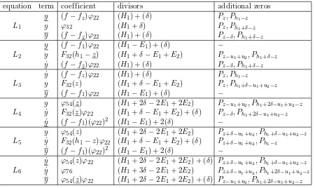
equation term coefficient divisors additional zeros
y (f−fz)ϕ22 (H1) + (δ) Pz, Ph1−z
L1 y ϕ32 (H1+δ) Pz, Ph1+δ−z
y (f−fz)ϕ22 (H1) + (δ) Pz−δ, Ph1+δ−z
y (f−f1)ϕ22 (H1−E1) + (δ) −
L2 y F32(h1−z) (H1+δ−E1+E2) Pz−u1+u2, Ph1+δ−z ˙
y (f−fz)ϕ22 (H1) + (δ) Pz−δ, Ph1+δ−z ˙
y (f−fz)ϕ22 (H1) + (δ) Pz, Ph1−z
L3 y F32(z) (H1+δ−E1+E2) Pz, Ph1+δ−u1+u2−z
y (f−f1)ϕ22 (H1−E1) + (δ) −
y ϕ54(z) (H1+ 2δ−2E1+ 2E2) Pz−u1+u2, Ph1+2δ−u1+u2−z
L4 y˙ F32(z)ϕ22 (H1+δ−E1+E2) + (δ) Pz−δ, Ph1+2δ−u1+u2−z ˙
y (f−f1)(ϕ22)2 (H1−E1) + 2(δ) −
y ϕ54(z) (H1+ 2δ−2E1+ 2E2) Pz+δ−u1+u2, Ph1+δ−u1+u2−z
L5 y˙ F32(h1−z)ϕ22 (H1+δ−E1+E2) + (δ) Pz+δ−u1+u2, Ph1−z ˙
y (f−f1)(ϕ22)2 (H1−E1) + 2(δ) − ˙
y ϕ54(z)ϕ22 (H1+ 2δ−2E1+ 2E2) + (δ) Pz+δ−u1+u2, Ph1+δ−u1+u2−z
L6 y˙ ϕ76 (H1+ 3δ−2E1+ 2E2) Pz+δ−u1+u2, Ph1+2δ−u1+u2−z ˙
y ϕ54(z)ϕ22 (H1+ 2δ−2E1+ 2E2) + (δ) Pz−u1+u2, Ph1+2δ−u1+u2−z Step 1:
Lemma 11. The Lax equationL3= 0 is uniquely characterised by the following properties:
(L3a) L3 ∈Φ332(P1P3· · ·P8PzPh1+δ−z−u1+u2|P1),
Proof . The property (L3b) follows directly from the corresponding conditions in (L1b) and (L2b). Let us consider the property (L3a). We know that the Lax equations (L1), (L2) have the following form:
(L1) L1= (f−fz)ϕ22y+F y+∗(f −fz)ϕ22y= 0, (L2) L2= (f−f1)ϕ22y+F′y+∗(f −fz)ϕ22y˙= 0.
Here F, F′ are some polynomials of degree (3,2) and ∗ represent some constant independent of (f, g). From the equation (f −f1)L1 −(f −fz)L2 = 0, we have three term relation bet-weeny,y, ˙y. This relation is apparently of degree (4,2), however, it is divisible byf−fz. Since
if it is not so, then it follows thaty= 0 forf =fz and for anyg, which contradict the 2nd
con-ditions of (L1b), (L2b). Then the quotient should belong to Φ332(P12P3· · ·P8Pz|Ph1+δ−z−u1+u2) as desired. Uniqueness follows by a simple dimensional argument as before.
The coefficients in (L2), (L3) are related as follows.
Lemma 12. For the normalized equations
(L2) y−A2(z)y+B2(z) ˙y= 0,
(L3) y−A3(z)y+B3(z) ˙y= 0,
we have
A3(h1+δ−z) =A2(z), B3(h1+δ−z) =B2(z).
Proof . This is because that the characterization properties (L2) and (L3) are related byy↔y
and z↔h1+δ−z.
Step 2:
Lemma 13. The Lax equationL4= 0 has the following characterizing properties:
(L4a) L4 ∈Φ354(P13P32· · ·P82Pz−u1+u2Ph1+2δ−z−u1+u2|P1),
(L4b) passing through 2 more points: Qu1 in (13) and Q˙z defined by ˙
Qz ={f˙=fz} ∩ {( ˙g−gh1−z) ˙y= ( ˙g−gz) ˙y}. (23)
Proof . Eliminating y from (L2) and (L3), one get three term relation between y, ˙y, ˙y. It is
apparently of degree (6,4) but divisible byf −fz. It is easy to check that quotient L4 belongs to Φ3
54(P13P32· · ·P82Pz−u1+u2Ph1+2δ−z−u1+u2|P1).
The first condition in (L4b) is the direct consequence of (L2b) or (L3b).
We will show the second condition in (L4b). Using the Lemma12, the (L4) equation can be written as
Ky+A2(z′)B2(z) ˙y+B2(z′) ˙y = 0, where z′ = h
1+ 2δ−z (i.e. z+z′ =h1) and the coefficient of y is K = 1−A2(z)A2(z′). By tracing the zeros, we see that the numerator of K is proportional to
ϕ54(z)∈Φ154 P14P32· · ·P82Pz−u1+u2Ph1+2δ−z−u1+u2
.
Hence, by Lemma 3, we have K= 0 when ˙f =fz. Thus, we have
˙
y
˙
y =−b(z)A2(z
′) for f˙=f
z.
Here, we put b(z) = B2(z)
A2(z′)|f˙=fz is evaluated as follows. By Lemma 5, we have A2(z;f, g) = A2(z; ˙f ,g˜˙). Hence,
by using the condition (L2b), we have
A2(z)|f˙=fz =
This is the desired 2nd relation in (L4b).
Step 3:
Lemma 14. The Lax equationL5= 0 has the following characterizing properties:
(L5a) L5 ∈Φ354(P13P32· · ·P82Pz+δ−u1+u2Ph1+δ−z−u1+u2|P1),
(L5b) passing through 2 more points: Qu1 in (13) and Q˙z defined by ˙
Qz ={f˙=fz} ∩ {( ˙g−gh1−z) ˙y= ( ˙g−gz) ˙y}. (27)
The proof is omitted since it is almost the same as Step 2.
Step 4:
Lemma 15. The Lax equationL6= 0 has the following characterizing properties:
(L6a) L6 ∈Φ376(P15P2P33· · ·P83Pz+δ−u1+u2|Ph1+2δ−z−u1+u2), (L6b) passing through 2 more points: Q˙z in (27) and Q˙z in (23).
Proof . Eliminatingy from equations
(L4) ϕ54(z)y+∗A32(z)ϕ22y˙+∗(f−f1)(ϕ22)2y˙= 0, (L5) ϕ54(z)y+∗A32(h1−z)ϕ22y˙+∗(f −f1)(ϕ22)2y˙ = 0,
we have ϕ54(z)L4 − ϕ54(z)L5 = 0. Which is apparently of degree (10,8) but divisible by (f−f1)ϕ22, hence we have the equation of degree (7,6). The vanishing conditions follows
Now we have the main result of this paper:
Theorem 1 (The compatibility). The equation(L6) is equivalent with equation(L1)evolved
by the translation TE2−E1:
ui7→u˙i, y7→y,˙ (f, g)7→( ˙f ,g˙).
Namely, the Lax pair (L1),(L2) is compatible if and only if the variables(f, g) solve the elliptic Painlev´e equation for T =TE2−E1.
Proof . We have obtained the characterization properties of (L6), hence our task is to compare
it with that forT(L1).
From these two conditions, we see thatT(L1) satisfy the condition (L6a) in Lemma15. The condition (L6b) is exactly the condition (L1b) transformed by T.
A
Discussion on the dif ferential case
In this appendix, we will discuss the differential case, taking the sixth Painlev´e equation PVI as an example. The PVI equation has a Hamiltonian form
dq
The equation (28) describes the iso-monodromy deformation of the Fuchsian differential equation on P1\ {0,1, t,∞}: These equations (30), (31) can be viewed as a Lax pair for thePVIequation. To see the geometric meaning of these Lax equations, let us introduce homogeneous coordinates (X:Y :Z)∈P2 by
q = Z
Z−X, p=
Y(Z−X)
XZ .
Proposition 2. The equation (30)can be uniquely characterized as an algebraic curveF(X,Y ,Z) = 0 of degree 4 in P2, satisfying the following vanishing conditions:
F(0,0,1) =F(1,−a2,1) =F(1,0,0) =F(0, a3,1) =F(1,−a1−a2,1) =F(1, a4,0) = 0,
Similarly the second Lax equation (31) has also a similar characterization as an algebraic curve
R(X, Y, Z) = 0 of degree 2 with the following conditions:
This geometric characterization of the Lax equations forPVImay be considered as a degener-ate case of our construction. The above result bear resemblance to the geometric characterization of the Hamiltonian H (29) as a cubic pencil [9].
Finally, let us give a comment on the apparent singularity and the non-logarithmic property. The Hamiltonian H in equation (29) is usually fixed by non-logarithmic condition for equa-tion (30) at the apparent singularity z =q. Namely, though the differential equation (30) has apparent singularity at z = q with exponents 0 and 2, the solutions are actually holomorphic there. In the difference Lax equation (L1) defined in Definition2, the factor (f−fz) or (f−fz) in
its coefficients looks like an “apparent singularity”. Since the non-logarithmicity is an essential property of the differential equation (30), it will be interesting if one can find the corresponding notion in difference cases.
Acknowledgements
The idea of this work came from the study of the Pad´e approximation method to the Painlev´e equations [13], and it was partially presented at the Workshop “Elliptic Integrable Systems, Isomonodromy Problems, and Hypergeometric Functions” [14]. The author would like to thank the organisers and participants for their interest. He also thank to Professors K. Kajiwara, T. Masuda, M. Noumi, Y. Ohta, H. Sakai, M-H. Saito and S. Tsujimoto for discussions. The author would like to thank the referees for their valuable comments and suggestions. This work is supported by Grants-in-Aid for Scientific No.17340047.
References
[1] Arinkin D., Borodin A., Moduli spaces ofd-connections and difference Painlev´e equations,Duke Math. J. 134(2006), 515–556,math.AG/0411584.
[2] Arinkin D., Borodin A., Rains E., Talk at the SIDE 8 workshop (June, 2008) and Max Planck Institute for Mathematics (July, 2008).
[3] Arinkin D., Lysenko S., Isomorphisms between moduli spaces of SL(2)-bundles with connections on P1\ {x1, . . . , x4},Math. Res. Lett.4(1997), 181–190.
Arinkin D., Lysenko S., On the moduli of SL(2)-bundles with connections on P1
\ {x1, . . . , x4},Internat. Math. Res. Notices1997(1997), no. 19, 983–999.
[5] Borodin A., Discrete gap probabilities and discrete Painlev´e equations,Duke Math. J.117(2003), 489–542, math-ph/0111008.
Borodin A., Isomonodromy transformations of linear systems of difference equations,Ann. of Math. (2)160 (2004), 1141–1182,math.CA/0209144.
[6] Grammaticos B., Nijhoff F.W., Ramani A., Discrete Painlev´e equations, in The Painlev´e Property: One Century Later, Editor R. Conte,CRM Ser. Math. Phys., Springer, New York, 1999, 413–516.
[7] Jimbo M., Sakai H., Aq-analog of the sixth Painlev´e equation,Lett. Math. Phys.38(1996), 145–154. [8] Kajiwara K., Masuda T., Noumi M., Ohta Y., Yamada Y.,10E9 solution to the elliptic Painlev´e equation,
J. Phys. A: Math. Gen.36(2003), L263–L272,nlin.SI/0303032.
[9] Kajiwara K., Masuda T., Noumi M., Ohta Y., Yamada Y., Cubic pencils and Painlev´e Hamiltonians, Funkcial. Ekvac.48(2005), 147–160,nlin.SI/0403009.
[10] Murata M., New expressions for discrete Painlev´e equations, Funkcial. Ekvac. 47 (2004), 291–305, nlin.SI/0304001.
[11] Rains E., An isomonodromy interpretation of the elliptic Painlev´e equation. I,arXiv:0807.0258.
[12] Sakai H., Rational surfaces with affine root systems and geometry of the Painlev´e equations,Comm. Math. Phys.220(2001), 165–221.
[13] Yamada Y., Pad´e method to Painlev´e equations,Funkcial. Ekvac., to appear.