Well-balanced computations of weak local residuals for the shallow water equations.

(1)

ANZIAM J. 56 (CTAC2014) pp.C128–C147, 2015 C128

Well-balanced computations of weak local

residuals for the shallow water equations

Sudi Mungkasi

1

Stephen G. Roberts

2

(Received 2 March 2015; revised 30 November 2015)

Abstract

The one-dimensional shallow water equations describe mass con-servation and momentum concon-servation. We propose a well-balanced numerical technique for computing weak local residuals of the momen-tum equation. We compare the performance of weak local residuals of the momentum equation to those of the mass equation. All weak local residuals behave similarly.

Introduction

Karni, Kurganov and Petrova [5] originally proposed using weak local residuals (or local truncation errors) as smoothness indicators for conservation laws. The available theory supporting weak local residuals as smoothness indicators is only valid for scalar conservation laws, but with numerical experiments weak local residuals as smoothness indicators were seen to be also valid for systems of conservation laws [4, 5]. A conservation law is homogeneous and so does not have any source terms. Section2 derives the weak local residual for the scalar balance law.

(3)

and Roberts [9] discussed measuring the smoothness of water height using mass conservation. In Section 3 we describe our numerical technique for computing the weak local residuals of the momentum equation.

Due to the existence of a source term in the momentum equation (equation of momentum conservation), the computation of the equation’s weak local residuals must be well-balanced. A non-well-balanced computation of a weak local residual may lead to spurious oscillations of the residual, leading to incorrect smoothness or error indicators. In this article we consider the steady state of a lake at rest. We develop well-balanced treatments for two different weak local residuals of the momentum equation. In addition, a wet/ dry interface treatment is also given in order to maintain the well-balanced property at wet/dry interfaces. Section 4 provides numerical tests for the performance of the weak local residuals.

2

Weak local residuals for balance laws

Kurganov et al. [4, 5] formulated the weak local residuals for conservation laws. These conservation laws are homogeneous, that is, they do not have source terms. We extend the work of Kurganov et al. [4, 5] to formulations of the weak local residuals of balanced laws. Balanced laws are conservation laws with additional nonzero source terms.

Consider the scalar balance law

qt+f(q)x =s, −∞< x <∞,

q(x,t) =q0(x), t=0.

(1)

Here x is a one-dimensional space variable, t is the time variable, q is the concentration of a quantity of interest,fis the flux ofq,sis a source function and q0 is an arbitrary function which defines the initial condition of q. Here

(4)

problem (1) is

Z∞

0

Z∞

−∞

[q(x,t)Tt(x,t) +f(q(x,t))Tx(x,t) +s(x,t)T(x,t)]dx dt

+

Z∞

−∞

q0(x)T(x,0)dx=0, (2)

where T(x,t)is an arbitrary test function. A mathematical derivation of this weak form was derived by Knobel [6] and Smoller [12].

Given a fixed spatial step∆xand temporal step∆t, we form a uniform spatial/ temporal grid made up of discrete spatial pointsxj:= j∆xfor j=0,1, . . . ,M and temporal points tn _:= _n∆t _for _n ₌ ₀_,₁_{, . . . ,}_N_{. We denote} _qn

j as the approximate value of q(xj,tn₎ _{computed by a conservative method. Like} Karni and Kurganov [4], we denote the corresponding piecewise constant approximation as

q∆(x,t) := qjn if (x,t)∈[xj−1/2,xj+1/2]×[tn−1/2,tn+1/2], (3)

where xj±1/2 := xj ±∆x/2 and tn±1/2 := tn ±∆t/2. We construct a test function T_jn(x,t) := Bj(x)Bn(t), where Bj(x) and Bn(t) are quadratic B-splines centered at x = xj and t = tn with supports of size 3∆x and 3∆t. That is,

Bj(x) =

             1 2 _x−x j−3/2 ∆x

2

if xj−3/2 6x6xj−1/2, 3

4 − x−xj

∆x 2

if xj−1/2 6x6xj+1/2,

1 2

_x−x j+3/2 ∆x

2

if xj+1/2 6x6xj+3/2,

0 otherwise,

(4)

and

Bn(t) =

             1 2

t−tn−3/2 ∆t

2

if tn−3/2 ₆_t₆_tn−1/2_, 3

4 − t−tn

∆t 2

if tn−1/2 ₆_t₆_tn+1/2_,

1 2

t−tn+3/2 ∆t

2

if tn+1/2 ₆_t₆_tn+3/2_,

0 otherwise.

(5)

Then substituting the test function Tjn(x,t) into (2) leads to a weak form of the local residual [4,5] for the balance law

En_j = −

Ztn+3/2

tn−3/2

Zx_j+3/2

x_j−3/2

q∆(x,t)

T_jn(x,t) t

+f(q∆(x,t))

T_jn(x,t) x+s

∆₍_x

,t)T_jn(x,t) dx dt. (6)

The weak local residual (6) is then

En_j = ∆x 12

qn+1 j+1 −q

n−1

j+1 +4 q n+1 j −q

n−1 j

+qn+1

j−1 −q n−1 j−1

+∆t

12

f(qn+1

j+1) −f(q n+1

j−1) +4 f(q n

j+1) −f(qnj−1)

+f(qn−1_j+1) −f(q

n−1 j−1)

−∆x∆t

36

sn−1_j−1 +4sn_j−1+s n+1 j−1

+4 sn−1_j +4sn_j +sn+1_j

+ sn−1_j+1 +4sn_j+1+s

n+1 j+1

. (7)

Using quadratic B-splines in constructing the test function is an adaption of the work of Karni, Kurganov, and Petrova [5] on conservation laws. So we refer to the weak local residual (7) as kkp (Karni–Kurganov–Petrova).

Rather than quadratic B-splines, we can also choose localized linear B-splines as the test functions T_jn−1/2+1/2 (x,t) := Bj+1/2(x)B

n−1/2₍_t₎_{, where} _B

j+1/2(x) and Bn−1/2(t) are centered at x = xj+1/2 and t = tn−1/2 with supports of size 2∆x and 2∆t. That is,

Bj+1/2(x) =

  

 

x−x_j−1/2

∆x if xj−1/26x 6xj+1/2, x_j+3/2−x

∆x if xj+1/26x 6xj+3/2,

0 otherwise,

(8)

and

Bn−1/2(t) =

  

 

t−tn−3/2 ∆t if t

n−3/2 ₆_t₆_tn−1/2_, tn+1/2_−t

∆t if t

n−1/2 ₆_t₆_tn+1/2_,

0 otherwise.

(6)

This results in a less expensive computation of the weak local residual

En_j+−1/21/2 = −

Ztn+1/2

tn−3/2

Zx_j+3/2

x_j−1/2

q∆(x,t)hT_jn+−1/21/2 i

t+f(q ∆₍

x,t))hT_jn+−1/21/2 i

x

+s∆(x,t)T_j+1/2n−1/2dx dt, (10)

which after a straightforward computation becomes

En−1/2_j+1/2 = ∆x 2

qn_j −qn−1_j +qn_j+1−q n−1 j+1 + ∆t 2

f qn−1 j+1

−f qn−1

j

+f qn_j+1

−f qn_j

− ∆x∆t

4

sn−1 j +s

n j +s

n−1 j+1 +s

n j+1

. (11)

Using linear B-splines to construct the test function is an adaption of the work of Constantin and Kurganov [3] on conservation laws. So we refer to the weak local residual (11) as ck (Constantin–Kurganov).

3

Shallow water equations

The shallow water equations are

ht+ (hu)x = 0, (12)

(hu)t+ hu2+ 1₂gh2

x = −ghzx. (13)

Here, x is the coordinate in one-dimensional space, t is time, u(x,t)denotes the water velocity, h(x,t) denotes the water height, z(x) is the topography, andg is the acceleration due to gravity. Another quantity of interest is the stage w=w(x,t) which is the water surface elevation given by w=h+z.

(7)

indicators for balance laws may lead to spurious oscillations of the indicator values. We show an example of this problem in Section 4. The problem is caused by source terms in the balance laws. To make the indicators work properly, we need to make the computation of the indicators well-balanced.

Mungkasi and Roberts [9] presented weak local residuals of the mass equation (equation of mass conservation) as smoothness indicators. No well-balanced technique was needed in that case since the mass equation does not have a source term. In the next two subsections we focus on well-balancing the weak local residual of the non-homogeneous momentum equation. We limit our discussion on the well-balanced technique to the steady state of a lake at rest.

3.1

Well-balancing the weak local residual

We propose a well-balanced technique for computing weak local residuals of the non-homogeneous momentum equation (13) in wet regions.

Consider the non-homogeneous momentum equation (13) and the weak local residual (7). For the steady state of a lake at rest, the weak local residual (7) simplifies to

Enj =

∆t 12

f(qn+1

j+1) −f(q n+1 j−1)

−∆x∆t

36

sn+1 j+1 +4s

n+1 j +s

n+1 j−1

+∆t

3

f(qnj+1) −f(q n j−1) − ∆x∆t 9

snj+1+4s n j +s

n j−1 +∆t 12

f(qn−1_j+1) −f(qn−1_j−1)

− ∆x∆t

36

sn−1_j+1 +4sn−1_j +sn−1_j−1

. (14)

In the case of a still lake f(qb a) =

1 2g(h

b

a)2. For our indicator to be well-balanced for the still lake case we need

[f(qj+1) −f(qj−1)] =

∆x

3 [sj+1+4sj+sj−1], (15)

(8)

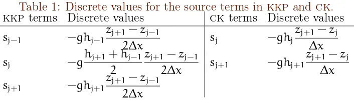
Table 1: Discrete values for the source terms in kkp and ck.

kkp terms Discrete values ck terms Discrete values

sj−1 −ghj−1

zj+1−zj−1

2∆x sj −ghj

zj+1−zj

∆x

sj −g

hj+1+hj−1

2

zj+1−zj−1

2∆x sj+1 −ghj+1

zj+1−zj

∆x sj+1 −ghj+1

zj+1−zj−1

2∆x

Since the fluxes in (15) are defined at the (j−1)th and (j+1)th cells, we need to enforce that the source term discretisations involve only the (j−1)th and (j+1)th cells. That is, we take sj = ₂1(sj+1+sj−1). Equation (15) is then rewritten as

g 2

(hj+1)2− (hj−1)2

=∆x[sj+1+sj−1]. (16)

Next, we use the same value for the topography gradientzx in the formulations ofsj+1 and sj−1, so that hj+1−hj−1 =zj−1−zj+1 for the lake at rest. This is achieved by discretising

(zx)j+1= (zx)j−1 := (zj+1−zj−1)/(2∆x). (17)

This last enforcement guarantees the well-balanced computation of the weak local residual (7). This source term discretisation technique is adapted from numerical schemes originally proposed by Bermudez and Vazquez [2]. This technique was also used by Audusse et al. [1] and Noelle et al. [10] to develop well-balanced numerical schemes. Each source term in kkp (7) and its discretisation using the above technique is given in the first and second column of Table 1, respectively.

(9)

3.2

Wet/dry interface treatment for the weak local

residual

The well-balanced technique describe in Section 3.1is valid for all-wet regions, that is, the(j−1)th,jth, and(j+1)th cells are wet. A numerical treatment at a wet/dry interface is needed and we describe it here. We omit the description of a dry/wet treatment, as it is similar to the treatment of a wet/dry interface.

We solve the shallow water equations using the finite volume method described by Mungkasi and Roberts [8]. We implement the discretisation proposed by Audusse et al. [1]. Quantities are reconstructed based on heighth, stage w:= h+z, and velocity u. We implement the wet/dry interface reconstruction, proposed by Audusse et al. [1]. The wet/dry interface reconstruction adjusts the bed topography z if negative water height occurs, so that the water height h remains nonnegative [1,8, for more details]. A second order method with a minmod limiter is used [11].

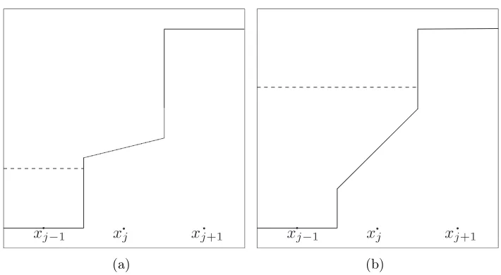
Since thekkpindicator of thejth cell involves three cells, namely the(j−1)th,

jth, and(j+1)th cells, there are two cases of the wet/dry interface for the kkpindicator: (a) wet-dry-dry, that is, wet for the (j−1)th cell, dry for the

jth cell, dry for the (j+1)th cell; and (b) wet-wet-dry, that is, wet for the

(j−1)th cell, wet for the jth cell, dry for the(j+1)th cell. These two cases are illustrated in Figure1. In the computation of thekkpindicator for these cases, zj+1 is replaced by wj−1. This ensures that the indicator computation at the wet/dry interface remains well-balanced. The two remaining special cases, namely wet-dry-wet and dry-wet-dry, are assumed to have indicator values of zero.

(10)

Figure 1: Two cases of the wet/dry interface for thekkpindicator: (a) the wet-dry-dry case; (b) the wet-wet-dry case. The dashed horizontal line indicates the water level.

(a) (b)

4

Numerical tests

We test the performance of weak local residuals. We use the second order well-balanced finite volume method [8]. Quantities are measured in siunits.

4.1

Well-balanced test

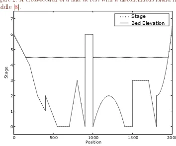
Consider a lake at rest with a discontinuous island in the middle of the lake, illustrated in Figure 2. This test is an adaptation of the test of Mungkasi and Roberts [8]. In the computation, the spatial domain is discretised into

800 cells.

(11)

Figure 2: A cross-section of a lake at rest with a discontinuous island in the middle [8].

Stage

Bed Elevation

0 500 1000 1500 2000

Position 0

1 2 3 4 5 6 7

S

ta

ge

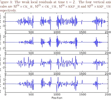
residuals of the mass and momentum equations based on (11), while kkp_h and kkp_uh are the weak local residuals of the mass and momentum equations based on (7). All indicators are the correct weak local residuals of the steady state of a lake at rest, correct to the order of10−15 (machine precision).

(12)

Figure 3: The weak local residuals at time t = 2. The four vertical axis scales are 1016_×_{ck_h}_,₁₀15_×_{ck_uh}_, ₁₀16_×_{kkp_h}_and₁₀15_×_{kkp_uh}_,

respectively.

0 500 1000 1500 2000

-3 0 3

10

^

16

C

K

h

0 500 1000 1500 2000

-2 0 2

10

^

15

C

Ku

h

0 500 1000 1500 2000

-2 0 2

10

^

16

K

Ph

0 500 1000 1500 2000

Position -1

0 1

10

^

15

K

Pu

(13)

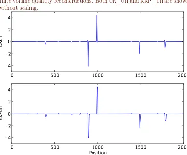
Figure 4: Unphysical weak local residuals at time t=2. Hereck_uh and

kkp_uh are computed naïvely using local cell quantity values based on

finite volume quantity reconstructions. Bothck_uh andkkp_uhare shown without scaling.

0 500 1000 1500 2000

−4 −2 0 2 4

C

Ku

h

0 500 1000 1500 2000

Position −4

−2 0 2 4

K

Pu

(14)

reconstructions. In this case, ck_uh and kkp_uh have large indicator values at some points, although these values should actually be zero.

4.2

Dam break test involving a dry area and moving

shock

Consider the collapse of a reservoir on a horizontal topography [9]

z(x) =0, 0 < x < 2000, (18)

with initial velocity and stage

u(x,0) =0, w(x,0) =

  

 

0 if 0 < x < 500,

10 if 500 < x < 1500,

5 if 1500 < x < 2000.

(19)

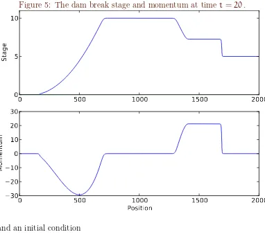
The simulation illustrates the motion of the water at any point x in the domain and at any time t > 0 with respect to the initial condition (19). Condition (19) describes two dam walls (at x=500 and x =1500). In the computation, the spatial domain is discretised into 800cells.

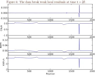
The simulation results at time t=20 are shown in Figures5and 6. Figure5

shows the stage and the corresponding momentum value. The weak local residualsck_h, ck_uh, kkp_h, andkkp_uh are shown in Figure 6. The ck_h indicator is best at identifying the shock.

4.3

Flow involving a stationary shock on an

obstruction

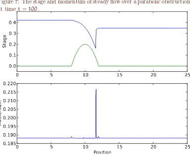
Consider a channel of length 25 with a parabolic bump topography [9]

z(x) =

0.2−0.05(x−10)2 if 86x 612,

(15)

Figure 5: The dam break stage and momentum at time t =20.

0

500

1000

1500

2000

0

5

10

Sta

ge

0

500

1000

1500

2000

Position

−30

−20

−10

0

10

20

30

Mo

me

ntu

m

and an initial condition

u(x,0) =0, w(x,0) =0.33, (21)

together with the Dirichlet boundary conditions

[w,hu,z,h,u] = [0.42,0.18,0.0,0.42,0.18/0.42] at x=0−

, (22)

[w,hu,z,h,u] = [0.33,0.18,0.0,0.33,0.18/0.33] at x=25+

. (23)

In the computation, the spatial domain is discretised into 400 cells.

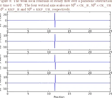
The simulation results at time t=100are shown in Figures7and8. Figure7

(16)

5 Conclusions C143

Figure 6: The dam break weak local residuals at time t=20.

0 500 1000 1500 2000

-0.015 0.000 0.015

C

K

h

0 500 1000 1500 2000

-1.0 -0.5 0.0

C

Ku

h

0 500 1000 1500 2000

0.00 0.06 0.12

K

Ph

0 500 1000 1500 2000

Position -2

-1 0

K

Pu

h

ck_h, ck_uh,kkp_h, and kkp_uh are shown in Figure 8. More details of these results are given by Mungkasi [7].

5

Conclusions

(17)

5 Conclusions C144

Figure 7: The stage and momentum of steady flow over a parabolic obstruction at timet =100.

0

5

10

15

20

25

0.0

0.1

0.2

0.3

0.4

Sta

ge

0

5

10

15

20

25

Position

0.185

0.190

0.195

0.200

0.205

0.210

0.215

0.220

Mo

me

ntu

m

shallow water equations, which are a system of balance laws. This suggests that weak local residuals may also be used as smoothness indicators for a system of balance laws in general, as long as an appropriate well-balanced treatment is used.

(18)

5 Conclusions C145

Figure 8: The weak local residuals of steady flow over a parabolic obstruction at timet=100. The four vertical axis scales are105_×_{ck_h}_,₁₀5_×_{ck_uh}_,

105_×_{kkp_h} _and ₁₀5_×_{kkp_uh}_{, respectively.}

0 5 10 15 20 25

-20 0 20

10

^

5

C

K

h

0 5 10 15 20 25

-10 0 10

10

^

5

C

Ku

h

0 5 10 15 20 25

-10 0 10

10

^

5

K

Ph

0 5 10 15 20 25

Position -10

0 10

10

^

5

K

Pu

(19)

References C146

References

[1] E. Audusse, F. Bouchut, M. O. Bristeau, R. Klein, and B. Perthame. A fast and stable well-balanced scheme with hydrostatic reconstruction for shallow water flows. SIAM J. Sci. Comput.25:2050–2065, 2004.

doi:10.1137/S1064827503431090. C135, C136

[2] A. Bermudez and M. E. Vazquez. Upwind methods for hyperbolic conservation laws with source terms. Comput. Fluids, 23:1049–1071, 1994. doi:10.1016/0045-7930(94)90004-3. C135

[3] L. A. Constantin and A. Kurganov. Adaptive central-upwind schemes for hyperbolic systems of conservation laws. In F. Asakura,

S. Kawashima, A. Matsumura, S. Nishibata, K. Nishihara (Eds.)

Hyperbolic problems: Theory, numerics, and applications. Vol. 1 of Proceedings of the 10th international conference, Osaka, Japan, 13–17 September 2004, Yokohama Publishers, Yokohama, 2006, pages 95–103, 2006. http://www.ybook.co.jp/pub/ISBN4-946552-21-9.htm,

http://129.81.170.14/~kurganov/Constantin-Kurganov.pdf C133

[4] S. Karni and A. Kurganov. Local error analysis for approximate

solutions of hyperbolic conservation laws. Adv. Comput. Math. 22:79–99, 2005. doi:10.1007/s10444-005-7099-8 C129, C130, C131,C132

[5] S. Karni, A. Kurganov, and G. Petrova. A smoothness indicator for adaptive algorithms for hyperbolic systems. J. Comput. Phys.

178:323–341, 2002. doi:10.1006/jcph.2002.7024 C129, C130, C132

[6] R. Knobel. An Introduction to the Mathematical Theory of Waves. American Mathematical Society, Providence, 2000.

http://www.ams.org/bookstore-getitem/item=stml-3 C131

(20)

References C147

Australian National University, Canberra, 2012.

http://hdl.handle.net/1885/10301 C143

[8] S. Mungkasi and S. G. Roberts. On the best quantity reconstructions for a well balanced finite volume method used to solve the shallow water wave equations with a wet/dry interface. ANZIAM J. 51:C48–C65, 2009

http://journal.austms.org.au/ojs/index.php/ANZIAMJ/article/

view/2576 C136, C137, C138

[9] S. Mungkasi and S. G. Roberts. Numerical entropy production for shallow water flows. ANZIAM J. 52:C1–C17, 2010. http://journal.

austms.org.au/ojs/index.php/ANZIAMJ/article/view/3786 C130,

C134, C141

[10] S. Noelle, N. Pankratz, G. Puppo, and J. R. Natvig. Well-balanced finite volume schemes of arbitrary order of accuracy for shallow water flows. J. Comput. Phy. 213:474–499, 2006. doi:10.1016/j.jcp.2005.08.019 C135

[11] P. L. Roe. Characteristic-based schemes for the Euler equations. Ann. Rev. Fluid Mech. 18:337–365, 1986.

doi:10.1146/annurev.fl.18.010186.002005 C136

[12] J. Smoller. Shock Waves and Reaction-Diffusion Equations.

Springer-Verlag, New York, 1983. doi:10.1007/978-1-4612-0873-0 C131