www.elsevier.nlrlocateraqua-online
Allozyme variation in three generations of selection
for whole weight in Sydney rock oysters
ž
Saccostrea glomerata
/
L.J. English
a,b,c, J.A. Nell
d, G.B. Maguire
b,e, R.D. Ward
a,b,)a
CSIRO Marine Research, GPO Box 1538, Hobart, Tasmania 7001, Australia
b
CooperatiÕe Research Centre for Aquaculture, GPO Box 1538, Hobart, Tasmania 7001, Australia
c
School of Aquaculture, UniÕersity of Tasmania, PO Box 1215, Launceston, Tasmania 7215, Australia
d
New South Wales Fisheries, Port Stephens Research Centre, Taylors Beach Road, Taylors Beach, NSW 2316, Australia
e
W.A. Marine Research Laboratories, Western Australia Fisheries, PO Box 20, North Beach, Western Australia 6020, Australia
Received 30 October 1999; received in revised form 15 July 2000; accepted 18 July 2000
Abstract
Genetic variability in second and third generations of a selective breeding line of Sydney rock
Ž .
oysters Saccostrea glomerata was compared with one another and a control group, using 14 allozyme loci. All groups showed a similar and high degree of genetic variability. Overall, the
Ž . Ž .
percentage of polymorphic loci P-0.99 criterion was 66.7%, the mean observed and expected
Ž . Ž .
heterozygosity "S.D. was 0.222"0.087 0.223"0.087 , and the mean number of alleles per
Ž .
locus "S.D. was 2.5"0.6. While selection for increased whole weight does not appear to have significantly diminished genetic variation of the two generations of the selected breeding line relative to the controls, there were some significant allele frequency differences among groups
Žns100 per group . Unexpectedly, the allele frequencies from the third-generation sample was.
more similar to those of the control sample than the second-generation sample, due to sampling error in the latter samples. This was reflected in estimated effective population numbers of 41.4"14.0 for the second-generation line and 383.8"249 for the third-generation lines, when compared to the control group, and 7.5"2 for the third generation when compared to the second generation. Numbers of alleles remaining in all cases were similar to numbers expected if allele
)Corresponding author. CSIRO Division of Marine Research, GPO Box 1538, Hobart, Tasmania 7001, Australia.
0044-8486r01r$ - see front matterq2001 Elsevier Science B.V. All rights reserved.
Ž .
( ) L.J. English et al.rAquaculture 193 2001 213–225
214
loss occurred through genetic drift or sampling variation only.q2001 Elsevier Science B.V. All
rights reserved.
Keywords: Saccostrea glomerata; Heterozygosity; Allozymes; Oysters; Australia
1. Introduction
Ž
Production of the native Sydney rock oyster, Saccostrea glomerata note species
Ž ..
name change from S. commercialis, see Anderson and Adlard 1994 , like many other native oysters, has declined in recent years. The Pacific oyster, Crassostrea gigas, now
Ž .
dominates world oyster production Shatkin et al., 1997 . Sydney rock oyster production has declined from about 14.5 million dozen oysters in the 1970s to 8.5 million dozen
Ž .
oysters in 1995r1996 NSW Fisheries, 1998 . Farming of the Sydney rock oyster,
Ž
which relies on natural spatfall, began on the Australian east coast New South Wales
. Ž
and southern Queensland in the 1870s and on the west coast in the early 1980s Nell,
.
1993 . Declining production rates have resulted from oyster mortalities by infection of
Ž
protoctistan parasites winter mortality, Mikrocytos roughleyi, and QX, Marteilia
.
sydneyi; Nell, 1993 , adverse effects of viral outbreaks among consumers, and
labour-in-tensive methods that have reduced economic viability.
In an attempt to increase profitability and to meet competition from the faster growing Pacific oyster in Tasmania, South Australia and New Zealand, a selective
Ž . Ž .
breeding program using mass selection was established in 1990 Nell et al., 1996 . Equal numbers of oysters were taken from each of four estuaries in New South Wales:
Ž X X
that only locally caught oysters were sampled, not those that had been transferred from another estuary. Oysters from each of the four estuaries were divided equally between
Ž .
eight groups for spawning 100 oystersrgroup . Of the 100 oysters in each of the eight spawning groups, not all of the 100 oysters spawned–only those that spawned profusely were used. Once oysters began to spawn, they were rinsed and continued to spawn in separate containers. Prior to fertilisation, all eggs were pooled separately for each mass spawning, and this process was repeated for all the sperm samples. The complete spawning procedure outlined previously was repeated for the spawning of subsequent generations. Control, or nonselected oysters, were taken from the same four estuaries as the original base population. An increase in whole weight of 18% was gained by the
Ž .
third generation Nell et al., 1999 . Production of triploid Sydney rock oysters rates has also been examined for its potential for increasing whole weight and it was found that triploid oysters were on average 41% heavier than their diploid counterparts after 2.5
Ž .
years of growth Nell et al., 1994 .
Selective breeding programs may result in the loss of genetic variation through
Ž .
inadequate numbers of parents, leading to inbreeding Tave, 1993 . Farming has led to
Ž .
the reduction of genetic diversity in Pacific oysters C. gigas in the United States of
Ž . Ž .
America Hedgecock and Sly, 1990 and in United Kingdom Gosling, 1982 .
Hedge-Ž .
were several orders of magnitude smaller than the number of broodstock actually used by industry. In Tasmania, farming has not led to the loss of appreciable amounts of
Ž .
genetic variation English et al., 2000 .
A previous study of Sydney rock oysters from three sites in New South Wales found
Ž .
heterozygosities ranging from 0.17 to 0.19 Buroker et al., 1979a . Ours is the first study to examine the genetic variability in a selected line. Allozyme electrophoresis was used to determine the levels of genetic diversity of the second- and third-generation oysters and of a control, unselected, line.
2. Methods
2.1. Sample collection
Ž
A mass selection program was set up in Port Stephens, New South Wales Nell et al.,
.
1996 . Spawning numbers for each of the groups are shown in Table 1. Samples of adductor muscle from approximately 100 individuals from each of a control line and the
Ž
second and third generations of the slat 2 Georges River Sydney rock oyster line Nell et
.
al., 1996 were air-freighted on dry ice to the laboratory, where all samples were stored
Ž
at y808C. Equal numbers of oysters from the same four estuaries Georges River,
.
Hawkesbury River, Port Stephens, Wallis Lake that founded the original base
popula-Ž .
tion were used as the control group Nell et al., 1996 , and were sampled for this study at the same time as the second generation of the selected line. No samples of the original controls or the first generation were analysed in this study as no oysters from these groups had been saved.
2.2. Allozyme analysis
Ž . Ž .
Eleven enzymes 13 loci and one general protein locus Table 2 were examined in
Ž .
about 100 oysters from each of the three groups. Adductor muscle about 200 mg was placed into separate 1.5-ml centrifuge tubes and homogenised in a few drops of distilled
water before being microcentrifuged for 10 min at 13,500=g. The supernatant was
subjected to cellulose acetate or starch gel electrophoresis. For cellulose acetate
elec-Table 1
Details of broodstock numbers used to found the various generations of S. glomerata Georges River Slat 2
Ž .
selection line and controls I. Smith, personal communication
Sample Spawning date No. of spawning Max. total number of
a groups used broodstock used
1st Generationrcontrol group February 1990 8 800
2nd Generation January 1992 3 22
3rd Generation January 1994 4 89
a
( ) L.J. English et al.rAquaculture 193 2001 213–225
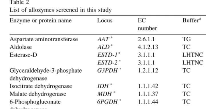
216 Table 2
List of allozymes screened in this study
a b
Enzyme or protein name Locus EC Buffer Time Structure
Ž .
number min
)
Aspartate aminotransferase AAT 2.6.1.1 TG 35 dimer
) Ž .
Aldolase ALD 4.1.2.13 TC 45 invariant
)
Esterase-D ESTD-1 3.1.1.1 LHTNC 300 dimer
)
ESTD-2 3.1.1.1 LHTNC 300 dimer )
Glyceraldehyde-3-phosphate G3PDH 1.2.1.12 TC 80 tetramer?
dehydrogenase
) Ž .
Isocitrate dehydrogenase IDH 1.1.1.42 TC 70 invariant
)
Malate dehydrogenase MDH 1.1.1.37 TC 90 dimer
)
6-Phosphogluconate 6PGDH 1.1.1.44 TC 90 dimer
dehydrogenase
)
Phosphoglucose isomerase PGI 5.3.1.9 LHTNC 300 dimer
)
Peptidase PEPS-1 3.4.11r13? TG 35 dimer
)
PEPS-2 3.4.11r13? TG 35 dimer
)
General protein PROT – TG 35 monomer
) Ž .
Superoxide dismutase SOD-1 1.15.1.1 LHTNC 300 invariant
)
SOD-2 1.15.1.1 LHTNC 300 dimer
a Ž .
TCstris citrate, TGstris glycine, LHTNCsL-Histidinertrisodium citrate starch . b
Subunit structure determined from heterozygote band patterns — note that G3PDH) heterozygotes were diffuse and the five bands expected of a tetramer could not be resolved.
trophoresis, Helena Titan III cellulose acetate plates were used with either a tris glycine
Ž0.02 M tris, 0.192 M glycine. or a 75-mM tris citrate ŽpH 7.0. buffer system
ŽRichardson et al., 1986; Hebert and Beaton, 1989 . The tris glycine gels were.
Ž .
electrophoresed at 200 V, the tris citrate gels at 150 V Table 2 . For starch gel electrophoresis, small pieces of Whatman No. 3 chromatography paper were soaked in the supernatant and placed in a gel made of 8% Connaught hydrolysed starch in a 5 mM
Ž .
L-Histidine HCl buffer pH adjusted to 7.0 with 0.1 M sodium hydroxide . The starch
Ž
gels were electrophoresed in 0.41 M trisodium citrate electrode buffer pH adjusted to
. Ž
7.0 with 0.5 M citric acid at 100 V. Standard enzyme staining protocols Richardson et
.
al., 1986; Hebert and Beaton, 1989 were used; the peptidase stains used glycyl-leucine
ŽPEPS-1). and phenylalyl-proline ŽPEPS-2). as substrates. General proteins were stained with Coomassie Blue.
Where an enzyme had multiple loci, the locus encoding the fastest migrating allozyme was designated ‘1’. Alleles within loci were numbered according to the anodal
Ž .
mobility of their product relative to that of the most common allele designated ‘100’ .
2.3. Data analysis
Mean sample sizes, numbers of alleles, heterozygosities and proportions of loci
Ž .
polymorphic were calculated by BIOSYS-1 Swofford and Selander, 1989 . Genetic
Ž .
Tests of conformation to Hardy–Weinberg equilibrium for each polymorphic locus in
Ž
each population used 1000 replicatesrtest of the CHIHW program Zaykin and
Pu-. wŽ .
dovkin, 1993 . The Selander index HobsyHexp rHexp, where Hobs and Hexp are
x
observed and Hardy–Weinberg expected heterozygosities, respectively was estimated and tested for loci showing a significant deviation from Hardy–Weinberg equilibrium, again using the CHIHW program. Allele frequency heterogeneity across populations was
Ž .
assessed using the CHIRXC program Zaykin and Pudovkin, 1993 . Both of these programs are based on Monte Carlo randomisations of the data, obviating the need to pool rare alleles.
To allow for multiple tests of the same hypothesis, Bonferroni corrections of the
preset significance level, a, were made by dividing a by the number of tests. For
example, where 11 variable loci were being tested at the 0.05 significance level, a
levels were reduced from 0.05 to 0.05r11s0.0045.
Ž .
The effective population sizes NK of the groups were estimated from allele
Ž . Ž .
frequency variances, using the methods of Pollak 1983 and Hedgecock and Sly 1990 .
The number of alleles at a given locus is k, F is the temporal allele frequency variancek
at a given locus, and FK is the multilocus estimate of allele frequency variance,
weighted by the number of independent alleles. As oysters from the control group were used as broodstock for the first generation, the control group oysters were considered the progenitors of second- and third-generation populations. When the control group was the
progenitor, the harmonic mean effective population sizes, N , values were calculated bye
Ž
multiplying NK by two, as there were two lines of descent control line and selected
Ž ..
line, see Hedgecock et al. 1992 . An analysis comparing the second and third
generations was also done, as oysters from the second generation were used directly as broodstock for the third generation. Data from loci that were monomorphic in all three
Ž .
groups ALD, IDH and SOD-2 were excluded from the calculations.
3. Results
Allele frequencies for the 14 isozyme loci were determined for control, second and
Ž .
third generations of selectively bred Sydney rock oysters Table 3 . Heterozygote
banding patterns for each of the enzymes showed the appropriate number of bands based
Ž . Ž .
on known subunit numbers Ward et al., 1992 . Three loci ALD, IDH, SOD-2 were
Ž .
invariant, and five loci 6PGDH, ESTD-2, G3PDH, PROT, SOD-1 showed only rare variants. The remaining six loci showed medium to high levels of variability. Genetic
Ž .
variability levels were determined for each group Table 4 ; all were high and similar to one another. All alleles with sample frequencies of 0.2 or greater were present in all groups.
Tests of allele frequency differentiation among the three groups revealed that seven of the 11 variable loci — AAT, ESTD-2, 6PGDH, PEPS-1, PEPS-2, PGI and SOD-1
Ž .
— showed significant a reduced to 0.05r11s0.0045 interpopulation heterogeneity
2 Ž .
after x analyses Table 5 .
Allele frequencies of groups were compared pairwise to locate the sources of the
Ž . 2
( ) L.J. English et al.rAquaculture 193 2001 213–225
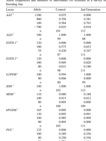
218 Table 3
Ž .
Allele frequencies and numbers of individuals n screened in a survey of a Sydney rock oyster selective breeding line
Locus Allele Control 2nd Generation 3rd Generation
)
AAT 1100 0.035 0.000 0.010
800 0.356 0.281 0.479
100 0.584 0.701 0.510
y700 0.025 0.018 0.000
n 101 112 97
)
ALD 100 1.000 1.000 1.000
n 99 88 97
)
ESTD-1 120 0.006 0.000 0.005
100 0.575 0.653 0.582
55 0.420 0.347 0.413
n 87 111 92
)
ESTD-2 120 0.000 0.000 0.016
100 0.969 0.820 0.964
80 0.031 0.180 0.021
n 98 111 96
)
G3PDH 100 0.994 1.000 1.000
80 0.006 0.000 0.000
n 80 99 98
)
IDH 100 1.000 1.000 1.000
n 102 112 95
)
MDH 110 0.080 0.188 0.106
100 0.915 0.812 0.889
80 0.005 0.000 0.006
n 100 109 90
)
6PGDH 165 0.005 0.000 0.000
130 0.005 0.091 0.005
100 0.985 0.909 0.990
80 0.005 0.000 0.005
n 102 111 99
)
PGI 125 0.006 0.000 0.035
100 0.289 0.256 0.260
PEPS-1 155 0.150 0.150 0.069
145 0.100 0.233 0.161
PEPS-2 110 0.029 0.014 0.028
100 0.676 0.804 0.608
90 0.276 0.173 0.318
80 0.018 0.009 0.045
Ž .
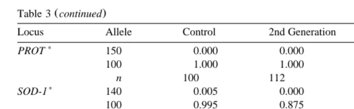
Table 3 continued
Locus Allele Control 2nd Generation 3rd Generation
)
PROT 150 0.000 0.000 0.006
100 1.000 1.000 0.994
n 100 112 79
)
SOD-1 140 0.005 0.000 0.000
100 0.995 0.875 1.000
50 0.000 0.125 0.000
n 102 112 99
)
SOD-2 100 1.000 1.000 1.000
n 103 112 112
Ž . Ž .
seven loci AAT, ESTD-2, MDH, 6PGDH, PEPS-2, PGI, SOD-1 between: a the
Ž .
second generation and both the control and third generation, and b across all groups.
PEPS-1 showed significant differences across all groups and between the second and
third generations. Genotype frequencies at all loci in all groups conformed to Hardy–
Ž
Weinberg equilibrium, except for the ESTD-2 locus in the second generation P
-. Ž
0.001 , which had a large and significant excess of homozygotes Selander index,
.
Ds y0.451, P-0.001 . Thus, significant allele frequency differences were observed
at seven loci between control and second generation, at eight loci between second and third generations, and at only one locus for control and third generation. This suggests that the second-generation sample is responsible for most of the heterogeneity observed.
Ž .
Unbiased genetic distances Nei, 1978 over 14 loci were estimated between pairwise
Ž
combinations of groups. All pairwise population distances are very small Nei, D
-.
0.013 . The genetic distance between the control and third generation is 0.0007, whereas the distance between these and the second generation is 0.0122.
Ž .
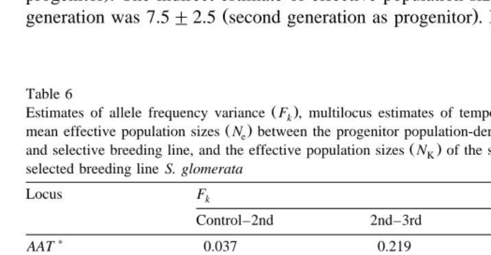
Temporal variation FK in allele frequencies was determined, and used to estimate
Ž . Ž .
effective population sizes NK and the expected number of alleles nt remaining in the
Ž .
populations as a result of random genetic drift Table 6 . The N of the third generationk
was calculated twice, once using the control group and once using the second generation as the progenitor population, to determine if the sampling variation in the
second-genera-Ž .
tion sample see Discussion would underestimate the NK value for the third generation.
One allele from the second generation and two alleles from the third generation were
Ž .
not seen in the control group Table 3 . Six alleles in the third generation were not present in the second-generation sample. Alleles that were not in the progenitor group
Ž .
were rare frequencies of less than 0.125 . These rare alleles were assumed to be present in the progenitor group but not detected in the sampling regime; they were omitted from
the calculations. Allele frequency variances, F , for variable loci, ranged from 0.007 tok
0.138 for the Control–2nd-generation analysis, from 0.006 to 0.250 for 2nd generation–
Ž .
3rd generation, and from 0.002 to 0.041 for Control–3rd generation Table 6 . The
weighted multilocus estimates of allele frequency variance, F , were lower for theK
Control–3rd-generation comparison, 0.019, than for those including the second
genera-Ž . Ž .
tion: 0.059 Control–2nd ; 0.077 2nd generation–3rd generation . The harmonic mean
Ž . Ž
()
L.J.
English
et
al.
r
Aquaculture
193
2001
213
–
225
220
Table 4
Ž .
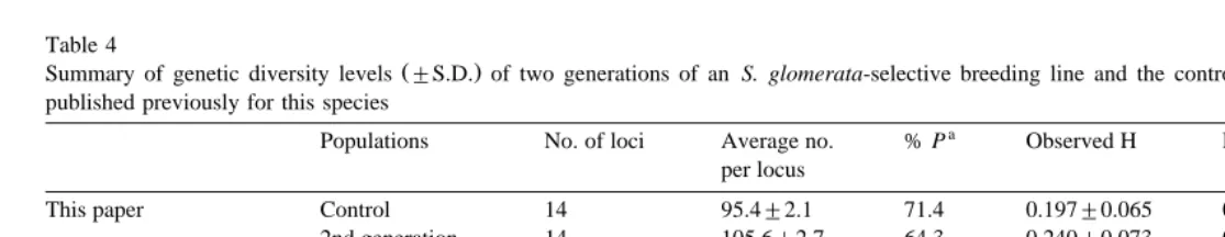
Summary of genetic diversity levels "S.D. of two generations of an S. glomerata-selective breeding line and the control line, and genetic diversity measures published previously for this species
a
Populations No. of loci Average no. % P Observed H Expected H Mean no.
per locus alleles
This paper Control 14 95.4"2.1 71.4 0.197"0.065 0.222"0.074 2.8"0.4
2nd generation 14 105.6"2.7 64.3 0.240"0.073 0.241"0.066 2.1"0.3 3rd generation 14 92.8"1.5 64.3 0.230"0.079 0.227"0.075 2.6"0.6 Mean 14 97.9"1.5 66.7 0.222"0.087 0.223"0.087 2.5"0.057
Ž .
Buroker et al. 1979a Tweed River 28 70.7 46.4 0.195"0.006 0.196"0.006 2.5
George’s River 28 79.3 46.4 0.172"0.006 0.184"0.006 2.5
Merimbula Lake 28 79.6 46.4 0.173"0.006 0.191"0.006 2.4
New Zealand 27 77.5 51.9 0.182"0.006 0.193"0.006 2.6
a
Table 5
Summary ofx2 analyses data for 11 variable loci for three S. glomerata populations 2
Locus Number n x Analysis
2
of alleles x P
)
AAT 4 310 31.220 -0.001
)
ESTD-1 3 305 4.219 0.441
)
ESTD-2 3 290 51.047 -0.001
)
G3PDH 2 277 2.467 0.307
)
MDH 3 299 13.067 0.007
)
6PGDH 4 312 33.453 -0.001
)
PGI 6 261 62.556 -0.001
)
PEPS-1 5 280 37.628 -0.001
)
PEPS-2 4 280 21.370 0.001
)
PROT 2 291 2.324 0.292
)
SOD-1 3 313 54.585 -0.001
.
generation varied considerably: 41.4"14.0 for the second-generation effective
popula-Ž . Ž
tion size Control as progenitor to 383.8"249 for the third generation Control as
. Ž .
progenitor . The indirect estimate of effective population size NK"S.D. for the third
Ž .
generation was 7.5"2.5 second generation as progenitor . Numbers of alleles
remain-Table 6
Ž . Ž .
Estimates of allele frequency variance F , multilocus estimates of temporal variance Fk K, the harmonic
Ž .
mean effective population sizes Ne between the progenitor population-derived population for control group
Ž .
and selective breeding line, and the effective population sizes NK of the second and third generation of the selected breeding line S. glomerata
Locus Fk
n and n : Numbers of alleles in the derived stocks expected given Nt o K and observed, respectively ignoring
.
( ) L.J. English et al.rAquaculture 193 2001 213–225
222
Ž
ing in the selective breeding lines were generally very similar to those expected Table
. Ž .
6 , given the estimated Nk effective population sizes .
4. Discussion
All groups — controls and two selected generations — of Sydney rock oysters
Ž
showed a high degree of genetic variability; overall variability levels about 68% of loci
.
polymorphic and average heterozygosities per locus around 0.22 were somewhat higher
Ž .
than in an earlier survey of this species that examined 28 loci Buroker et al., 1979a
ŽTable 4 . The differences may reflect real differences in variability among samples.
andror the use of different samples of loci and different electrophoretic techniques. The two generations of the selected line showed no reduction in genetic variation compared
Ž .
with the control group. Smith et al. 1986 made the same finding when comparing introduced New Zealand wild stocks of Pacific oysters with cultured oysters from
Ž .
Mangokuura, Japan. English et al. 2000 also found little reduction in genetic diversity when comparing hatchery and established Australian stocks with ancestral, native Japanese stocks. However, American and British hatchery stocks of Pacific oysters are
Ž . Ž
reported to have lost variation for AAT Hedgecock and Sly, 1990 and PGI Gosling,
.
1982 , respectively.
The reduction in mean numbers of alleles per locus in Sydney rock oyster populations from 2.8 in the controls to 2.1 in the second generation and 2.6 in the third generation, while not statistically significant, suggests that some allele loss might have occurred. The lower value for the second-generation sample is probably due to sampling variation alone. However, any loss of alleles could be examined further using hypervariable loci, such as microsatellites; such loci typically have far higher numbers of alleles per locus
Ž
and would be more powerful markers of genetic variation than allozymes Wright and
.
Bentzen, 1994; Reilly et al., 1999 .
Almost all genotype frequencies showed good agreement with Hardy–Weinberg expectations — the only exception was a significant heterozygote deficiency at ESTD-2
Ž .
in the second generation. Buroker et al. 1979a observed mean heterozygosities less than Hardy–Weinberg expectations, but these were not significant for two of their three
Ž .
sites including Georges River, a site contributing to the control group in this study . The conformation to Hardy–Weinberg expectations of almost all genotype frequencies
Ž .
observed in the present study Table 4 differ from studies of other oyster species, such
Ž
as C. gigas Buroker et al., 1975, 1979a,b; Fujio, 1979; Gosling, 1982; Smith et al.,
. Ž
1986; Moraga et al., 1989; Deupree, 1993; English et al., 2000 and C.Õirginica Singh
.
and Zouros, 1978; Zouros et al., 1980 , where heterozygosity deficits have been widely observed.
Ž .
oysters collected for the second-generation sample could not have been representative of the true genetic status of this line, and this sampling error has had a significant influence on estimates of gene diversity. While important, this effect is not very substantial: all
Ž .
pairwise Nei 1978 genetic distances between groups are -0.013.
Ž .
Effective population numbers NK can be estimated from temporal variance in allele
Ž
frequencies Pollak, 1983; Waples, 1989; Hedgecock and Sly, 1990; Hedgecock et al.,
.
1992 . The basic rationale is that the smaller the N , the larger the allele frequencyK
variance between generations. The second generation had six fewer alleles than the third
generation and may, therefore, underestimate the NK value for the third generation.
Also, given that the third generation appeared more similar genetically to the control
group in other calculations of genetic variability, the NK of third generation was also
calculated using the control group as the progenitor population. Comparing these results
Ž .
with the actual numbers of parents used I. Smith, personal communication , the mean
Ž .
effective population number Ne for the second generation, 41.4"14.0, is higher than
the maximum possible number of first-generation oysters contributing to the second
generation, 22. For the third generation, the estimated NK of 7.5"2.5 is substantially
lower than the maximum possible number of 89 second-generation oysters contributing
to the third generation. However, the estimated NK of 383.8"249 for the third
generation, using the controls as the progenitors, is substantially higher than the previous estimate, and higher than maximum possible number of immediate parents of 89. The control sample was collected contemporaneously with the second-generation sample, so has undergone one less generation than the third-generation sample, and this effect may
be inflating the N .e
This high N , together with the high Fe K values observed between the
tion oysters and the other populations, suggests that the sampling error in
second-genera-tion oysters is underestimating the NK of the third generation when using the
second-generation sample as progenitors. Estimated effective population sizes larger than the number of actual parents used have been observed in a hatchery stock of hard clams
ŽMercenaria mercenaria and four selected lines of pearl oysters Pinctada martensii. Ž .
ŽHedgecock et al., 1992 . On the other hand, Hedgecock and Sly 1990 found effective. Ž .
Ž
population sizes of two U.S. farmed stocks of Pacific oysters to be 40.6"13.9 Willapa
. Ž .
Bay and 8.9"2.2 Humboldt Bay , the latter stock having become fixed for an
otherwise rare allele at one locus, even though much larger numbers of broodstock are routinely used by industry.
Despite the difference between actual and estimated broodstock numbers, the ex-pected numbers of alleles of the second and third generations of the selected breeding line were very close to the observed numbers in all cases, suggesting that random
Ž .
genetic drift sampling variation alone was the cause of allelic variation between the
Ž .
groups. This was also true for two U.S. farmed stocks Hedgecock and Sly, 1990 of Pacific oysters, a hard clam hatchery stock and four selected lines of pearl oysters
ŽHedgecock et al., 1992 ..
( ) L.J. English et al.rAquaculture 193 2001 213–225
224
the second generation and other samples appears to be due to a sampling artifact; it is
Ž
likely to be biologically unimportant. The type of selective breeding program used mass
.
selection aided the retention of genetic diversity across the generations sampled. By using oysters from four different areas and using large numbers of oysters for spawning helped to achieve the levels of genetic diversity observed. Not all of the oysters collected for spawning actually spawned. But separating spawning oysters and by mixing equal amounts of each of the sperm and eggs, ensured that any given oyster’s sperm or eggs could not dominate the total amounts present, thereby could not homogenize the levels of genetic variability of the subsequent generation.
Acknowledgements
This project was funded by the Cooperative Research Centre for Aquaculture. The authors wish to thank the following for their assistance in the supply or collection of
Ž
oysters for this study: Rosalind Hand and Ian Smith NSW Fisheries, Port Stephens
.
Research Centre . We thank Drs. John Benzie, Nick Elliott and Peter Rothlisberg and three anonymous referees for comments on earlier versions of the paper.
References
Anderson, T.J., Adlard, R.D., 1994. Nucleotide sequence of a rDNA internal transcribed spacer supports synonymy of Saccostrea commercialis and S. glomerata. J. Molluscan Stud. 60, 196–197.
Buroker, N.E., Hershberger, W.K., Chew, K.K., 1975. Genetic variation in the Pacific oyster. J. Fish. Res. Board Can. 32, 2471–2477.
Buroker, N.E., Hershberger, W.K., Chew, K.K., 1979a. Population genetics of the family Ostreidae: I. Intraspecific studies of Crassostrea gigas and Saccostrea commercialis. Mar. Biol. 54, 157–169. Buroker, N.E., Hershberger, W.K., Chew, K.K., 1979b. Population genetics of the family Ostreidae: II.
Interspecific studies of the genera Crassostrea and Saccostrea. Mar. Biol. 54, 171–184.
Ž .
Deupree Jr., R.H., 1993. Genetic characterization of deep-cupped Pacific oysters Crassostrea gigas from Tasmania, Australia. Unpublished masteral thesis, University of Washington, Seattle, WA.
English, L.J., Maguire, G.B., Ward, R.D., 2000. Genetic variation of wild and hatchery populations of the
Ž .
Pacific oyster, Crassostrea gigas Thunberg , in Australia. Aquaculture 187, 283–298.
Fujio, Y., 1979. Enzyme polymorphism and population structure of the Pacific oyster Crassostrea gigas. Tohoku J. Agric. Res. 30, 32–42.
Ž .
Gosling, E.M., 1982. Genetic variability in hatchery-produced Pacific oysters Crassostrea gigas Thunberg . Aquaculture 26, 273–287.
Hebert, P.D.N., Beaton, M.J., 1989. Methodologies for Allozyme Analysis Using Cellulose Acetate Elec-trophoresis. Helena Laboratories, Beaumont, TX.
Hedgecock, D., Sly, F., 1990. Genetic drift and effective population sizes of hatchery-propagated stocks of the Pacific oyster, Crassostrea gigas. Aquaculture 88, 21–38.
Hedgecock, D., Chow, V., Waples, R.S., 1992. Effective population numbers of shellfish broodstock estimated from temporal variance in allelic frequencies. Aquaculture 108, 215–232.
Moraga, D., Osada, M., Lucas, A., Nomura, T., 1989. Genetique biochemique de populations de Crassostrea` `
Ž . Ž . w
gigas en France cote Atlantique et au Japon Miyagi . Biochemical genetics of Crassostrea gigasˆ
Ž . Ž .x
populations from France Atlantic coastline and from Japan Miyagi Aquat. Liv. Resour. 2, 135–143. Nei, M., 1978. Estimation of average heterozygosity and genetic distance from a small number of individuals.
Ž .
Nell, J.A., 1993. Farming the Sydney rock oyster Saccostrea commercialis in Australia. Rev. Fish. Sci. 1, 97–120.
Nell, J.A., Cox, E., Smith, I.R., Maguire, G.B., 1994. Studies on triploid oysters in Australia: I. The farming
Ž .
potential of triploid Sydney rock oysters Saccostrea commercialis Iredale and Roughley . Aquaculture 126, 243–255.
Nell, J.A., Sheridan, A.K., Smith, I.R., 1996. Progress in a Sydney rock oyster Saccostrea commercialis
ŽIredale and Roughley breeding program. Aquaculture 144, 295–302..
Nell, J.A., Smith, I.R., Sheridan, A.K., 1999. Third generation evaluation of Sydney rock oyster Saccostrea
Ž .
commercialis Iredale and Roughley breeding lines. Aquaculture 170, 195–203.
NSW Fisheries, 1998. 1997 NSW oyster industry report. Status of Fisheries Resources 1996r1997. NSW Fisheries, Sydney, 91.
Pollak, E., 1983. A new method for estimating the effective population size from allele frequency changes. Genetics 104, 531–548.
Reilly, A., Elliott, N.G., Grewe, P.M., Clabby, C., Powell, P., Ward, R.D., 1999. Genetic differentiation
Ž .
between Tasmanian cultured Atlantic salmon Salmo salar L. and their ancestral Canadian population: comparison of microsatellite DNA and allozyme and mitochondrial DNA variation. Aquaculture 173, 459–469.
Richardson, B.J., Braverstock, P.R., Adams, M., 1986. Allozyme Electrophoresis: A Handbook for Animal Systematics and Population Studies. Academic Press, Sydney, 410 pp.
Shatkin, G., Shumway, S.E., Hawes, R., 1997. Considerations regarding the possible introduction of the
Ž .
Pacific oyster Crassostrea gigas to the Gulf of Maine: a review of global experience. J. Shellfish Res. 16, 463–477.
Singh, S.M., Zouros, E., 1978. Genetic variation associated with growth rate in the American oyster
ŽCrassostreaÕirginica . Evolution 32, 342–353..
Smith, P.J., Ozaki, H., Fujio, Y., 1986. No evidence for reduced genetic variation in the accidentally introduced oyster Crassostrea gigas in New Zealand. N. Z. J. Mar. Res. 20, 569–574.
Swofford, D.L., Selander, R.B., 1989. BIOSYS-1: A Computer Program for the Analysis of Allelic Variation
Ž .
in Population Genetics and Biochemical Systematics Release 1.7 . Illinois Natural History Survey, Champaign, IL, 39 pp.
Tave, D., 1993. Genetics for Fish Hatchery Managers, 2nd edn. Van Nostrand-Reinhold, New York, pp. 216–217, 415 pp.
Waples, R.S., 1989. A generalized approach for estimating effective population size from temporal changes in allele frequency. Genetics 121, 379–391.
Ward, R.D., Skibinski, D.O.F., Woodwark, M., 1992. Protein heterozygosity, protein structure and taxonomic differentiation. Evol. Biol. 26, 73–159.
Wright, J.M., Bentzen, P., 1994. Microsatellites: genetic markers for the future. Rev. Fish Biol. Fish. 4, 384–388.
Zaykin, D.V., Pudovkin, A., 1993. Two programs to estimate significance of chi-square values using pseudo-probability tests. J. Hered. 84, 152.