SAR-based change detection using hypothesis testing and Markov random field modelling
Wenxi Cao a,*, Sandro Martinis a a
German Remote Sensing Data Center (DFD), German Aerospace Center (DLR), 82234 Oberpfaffenhofen, Germany *Corresponding author: [email protected], +49 8153 28 3384
Commission VI, WG VI/4
KEY WORDS: Three-Class Change Detection, Synthetic Aperture Radar (SAR), Post-Classification, Disaster Monitoring, Graph-Cut, Markov Random Field (MRF)
ABSTRACT:
The objective of this study is to automatically detect changed areas caused by natural disasters from bi-temporal co-registered and calibrated TerraSAR-X data. The technique in this paper consists of two steps: Firstly, an automatic coarse detection step is applied based on a statistical hypothesis test for initializing the classification. The original analytical formula as proposed in the constant false alarm rate (CFAR) edge detector is reviewed and rewritten in a compact form of the incomplete beta function, which is a built-in routbuilt-ine built-in commercial scientific software such as MATLAB and IDL. Secondly, a post-classification step is built-introduced to optimize the noisy classification result in the previous step. Generally, an optimization problem can be formulated as a Markov random field (MRF) on which the quality of a classification is measured by an energy function. The optimal classification based on the MRF is related to the lowest energy value. Previous studies provide methods for the optimization problem using MRFs, such as the iterated conditional modes (ICM) algorithm. Recently, a novel algorithm was presented based on graph-cut theory. This method transforms a MRF to an equivalent graph and solves the optimization problem by a max-flow/min-cut algorithm on the graph. In this study this graph-cut algorithm is applied iteratively to improve the coarse classification. At each iteration the parameters of the energy function for the current classification are set by the logarithmic probability density function (PDF). The relevant parameters are estimated by the method of logarithmic cumulants (MoLC). Experiments are performed using two flood events in Germany and Australia in 2011 and a forest fire on La Palma in 2009 using pre- and post-event TerraSAR-X data. The results show convincing coarse classifications and considerable improvement by the graph-cut post-classification step.
1. INTRODUCTION 1.1 Problem Description
Natural disaster can affect residence of human beings, cause economic damage and even take lives of thousands of people every year. It is essential to monitor natural disasters and to provide valid near real-time crisis information, so that rescue work can be conducted in time to keep the loss as less as possible. In this context Synthetic Aperture Radar (SAR) turns out to be an excellent sensor for disaster monitoring because of its ability of all-weather data acquisition. In view of this virtue it is valuable to develop appropriate algorithms to extract more information from SAR data. This study is dedicated to one of them called change detection.
Change detection is the process of identifying differences in the state of an object or phenomenon by observing it at different times (Lu et al., 2004). The goal of change detection is to detect "significant" changes while rejecting "unimportant" ones (Radke et al., 2005). In general significant changes may reflect natural phenomena or anthropogenic activities on the Earth’s surface. A typical application of change detection is to monitor abrupt changes caused by natural disaster and extract relevant crisis information to support crisis response and rescue work.
1.2 Related Works
There are many change detection techniques in the literature. Lu et al. (2004) and Radke et al. (2005) provide comprehensive reviews for the present methods. The following categories of change detection are summarised in (Lu et al., 2004):
1. Algebraic methods such as image differencing, image ratioing, image regression, vegetation index differencing, change vector analysis (CVA) and background subtraction. 2. Transformation methods like principal component analysis (PCA), Gramm-Schmidt and Chi-square transformations.
3. Classification methods for multi-spectral images such as post-classification comparison, spectral-temporal combined hybrid change detection and artificial neural network (ANN).
4. Advanced models, for example a biophysical model related to the scattering process of vegetation to find changed areas.
There is no ideal algorithm for all problems. Algebraic methods are efficient and easy to implement, but it is hard to find a suitable threshold to make an optimal classification. Other methods in the list above outperform the algebraic methods, but they are complex and time-consuming. This paper focuses on the application of SAR data in the field of disaster monitoring. For this purpose efficient algebraic methods are preferred in order to get near real-time information as soon as possible.
Despite of the convinced experimental results in these papers there are still some problems that are not so far discussed but inevitable for applications of SAR change detection in the field of natural disaster monitoring, such as:
1. Most of these methods only discuss a two-class problem, i.e. they only classify a pair of images into a changed and no-changed set of pixels. In general there are three classes in change detection: positive change, negative change and non-change. For example, in flood monitoring, flood and receding water areas should be classified into negative- and positive-change class. In case of partially submerged vegetation there are also frequently positive- and negative-changed classes to distinguish.
2. Most of the discussions in the literature are restricted in pixel-based thresholding algorithms. Because of speckle noise in SAR images, the effect of a pixel-based thresholding approach is limited regardless of which criterion for the optimal threshold is defined. Most of the methods filter SAR images before classification in order to reduce the speckle noise. However, many details in SAR images could be removed or modified by this processing step. In general, a post-classification step can be used to improve the coarse classification result obtained by thresholding (Radke et al., 2005).
1.3 Organisation of the Paper
In this paper we inherit the key ideas in the literature mentioned in subsection 1.2 to solve these two problems. Section 2 describes the proposed change detection method that consists of a coarse classification and a post-classification. In subsection 2.1 the hypothesis test for SAR-based change detection is at first reviewed and modified in a compact form using the incomplete beta function. In subsection 2.2 the concept of Markov Random Fields (MRF) is introduced to formulate the problem of post-classification. Afterwards a graph-cut algorithm is applied to solve this general optimization problem. The concrete energy functions for this algorithm are defined in this subsection. Section 3 reports on the results of the application of the proposed automatic method to SAR images acquired in many different disaster scenarios. At the end conclusions and outlook and drawn in Section 4.
2. METHODOLOGY
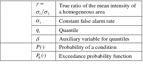
Before starting discussion on the proposed method in this study some notations used in this article are summarized in table 1 to provide an overview of involved physical variables.
Notation Variable
G Mean intensity of a homogeneous area in the i-th SAR image
n Speckle noise in SAR images
i
= Observed ratio of the mean
intensity of a homogeneous area
1 2
γ σ σ
= True ratio of the mean intensity of a homogeneous area
t
α Constant false alarm rate
t
q Quantile
δ Auxiliary variable for quantiles ( )
P⋅ Probability of a condition
E( )
P ⋅ Exceedance probability function
Table 1. Notations for variables
2.1 Initial Classification based on Hypothesis Test
2.1.1 Review of hypothesis test for SAR change detection: The one-sided hypothesis test for positive change detection is generally formulated as: geneous area in two coregistered SAR images, as listed in table 1. The constant false alarm rate αU describes the probability of rejecting H0 given that it is true. It can be formulated as:
U P( qU)
α = γ > (1.2)
Introducing an exceedance probability function defined by:
E( ) ( )
P q =P r>q (1.3)
the constant false alarm rate �U can further be related to the exceedance probability function by rewriting the quantile �Uas�U=��U:
The formulation above also applies to the corresponding one-sided hypothesis test for negative change detection. That provides:
Equation 1.4 and 1.5 enable us to calculate the corresponding quantiles with respect to certain constant false alarm rates �U,�L if a certain exceedance probability function �E(�) is defined. An example of �E(�) formulated by a series expansion is described in Oliver et al. (1996):
2.1.2 Ratio of Gamma random variables: Assuming that SAR images have been segmented into many homogeneous areas with pixel number��, the pixels in each area of the first image follow the same Gamma distribution:
1 1 1
Gamma( , ) for 1, 2, , i
X ∼ k θ i= N (1.7)
where �1,�1 are parameters for the Gamma distribution (Lindgren, 1993) that are constant for all pixels in a homogeneous area of the first SAR image. For a homogenous area in the second image the situation is similar:
2 2 2
Gamma( , ) for 1, 2, , j
X ∼ k θ j= N (1.8)
The parameterization of a Gamma function is different in statistics and SAR data processing. The parameters in Equation 1.7 and 1.8 are related to the parameters in table 1 by the following equation:
If an area of pixels has changed, there must be also a difference between their mean values. The task is now to find the PDF for the mean value of �Gamma distributed random variables. This can be solved based on following three properties of the Gamma distribution (Lindgren, 1993):
Table 2. Properties of Gamma distribution
The summation and the scaling property with �= 1/� provide:
1
where the last equation uses the third property specified in table 2. In addition, ��2 distribution is related to Fisher distribution by the following property:
Applying Equation 1.12 to Equation 1.10 provides:
1
With Equation 1.9 and the relation in table 1, equation 1.13 is equal to:
Using the true and observed ratio specified in table 1 to rewrite the equation 1.14 gives:
1 1 2 2
According to Pearson (1968), the cumulative distribution function CDF of F-distribution �(�; �1,�2) can be formulated commonly available built-in function of MATLAB or IDL. The exceedance probability function can then be described as:
( )
Combining equation 1.4, 1.5 and 1.17 provides:
1 1
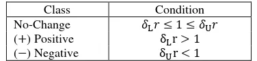
Given two constant false alarm rates�L,�U, the parameters �L,�Ucan be calculated from equation 1.18. Then the decision
rules for three-class change detection are:
Class Condition
No-Change �L� ≤1≤ �U�
(+) Positive δLr > 1
(−) Negative δUr < 1
There are many ways to apply equation 1.18 and the decision rules in Table 3. If �1=�2= 1, this method degenerates into a pixel-based one. It can be used to perform a quick coarse classification that provides a seed for the following post-classification. If �1> 1,�2> 1, this method is region-based. If a segmentation mask is available, this region-based method provides a way of direct classification without the need of any post-processing. The region-based version can also be applied to averaged and subsampled SAR images in order to reduce the process time. In this study we only use the hypothesis test as a pixel-based method to provide a seed for its post-classification. The purpose is to demonstrate the effect of the graph-cut algorithm on this coarse initial result.
2.2 Post-classification based on Markov Random Fields and Graph-Cuts
Classification results based on thresholding are generally liable to speckle noise in SAR images. This type of noise is an effect of most coherent imaging systems and results in a “dirty” classification. A post-processing step is necessary to reduce the randomness of the classification results due to the speckle noise in SAR images. As a classification result can be considered as a mask, in which each pixel is labeled with its class ID post-processing can be seen as correction of the initial classification of the image. In the literature this task is formulated in the frame of Markov random fields (MRF) (Li, 1995).
2.2.1 Markov Random Fields: Post-processing usually integrates priori knowledge in the classification step to improve the classification. One of the assumptions in MRF is that real objects are homogeneously distributed. Thus objects of the same category should almost gather together in images. Based on this consideration the expected classification result should be represented in areas or blocks instead pixels.
This idea of MRFs is formulated by two functions: data energy function and smoothness energy function. The data energy function focuses on the similarity of pixel values in each class. If pixels labeled in a class have similar values, they will receive low data energy values, and vice versa. In this way the data energy quantizes the quality of a certain classification. On the other hand, the smoothness energy function takes the neighborhood of pixels into consideration. Classifications with scattered regions of pixels have higher smoothness energy than those with connected regions of pixels. In this way the smoothness energy describes if the pixels of a same class clutter together or scatter randomly.
Mathematically the set of pixels in an image � is denoted as�0. A classification or labeling of this image is then denoted as �=���,∀� ∈ �0�where�� means the class label of pixel� ∈ potential. With these notations the whole energy of the MRF under the labeling � is described as: �(�) globally provided that the data and smoothness energy functions are suitably defined. In the literature there are many
algorithms to solve this general optimization problem, such as iterated conditional modes (ICM) (Besag, 1986) and simulated annealing (SA) (Geman et al., 1984). In the following an effective algorithm based on graph-cuts is applied to solve the optimization problem on a MRF.
2.2.2 Graph-cut Algorithm: A graph is composed of nodes and edges. Each edge in the graph can transport an amount of flow between its two nodes. The maximum of the flow is limited by the capacity of the edges. If the flow in one edge has reached its capacity, this edge is blocked and cannot transport flow anymore. The connection between the source and the sink nodes through edges forms a path for flow transport. The maximum of flow in this path (max-flow) is reached if the capacity of one edge in the path has been fully used. In this situation this path is called blocked. In order to find the max-flow from source to sink, every possible path should be fully used to transport flow until they are all blocked. Then the sum of flow in these paths is the maximal flow.
Another interesting viewpoint is given by Ford et al. (1956). According to their theorem the maximal flow in each path is only determined by those edges with minimal capacities, i.e. the blocked edges. So the max-flow in the whole graph is equal to the sum of capacities of the blocked edges. In addition, these blocked edges cut the graph into two parts. One part is connected with the source, denoted as��, the other is connected to the sink, denoted as��. The blocked edges are the channel of these two parts. In the case of max-flow, the capacities of the blocked edges are fully used and determine the maximal flow. In this viewpoint Ford et al. (1956) equates the max-flow with the best cut of a graph. Since there are many possible cuts which divide the graph into two parts��,��, the best cut is so defined that the sum of capacities of the cut edges is minimal (min-cut). These cut edges are equivalent to the blocked edges in the max-flow problem.
Kolmogorov et al. (2004) transforms the optimization problem on a two-class MRF to the problem of max-flow/min-cut in a graph. The purpose of the transformation is to benefit from some global optimization methods in the graph theory. Boykov et al. (2004) apply the graph construction method in Kolmogorov et al. (2004) to a multi-label graph and proposes a novel algorithm to perform max-flow optimization. According to their experiments their new method significantly outperforms other standard algorithms. In this study we use the graph-cut and max-flow methods by Kolmogorov et al. (2004) and Boykov et al. (2004) to solve the optimization problem on a MRF. Their algorithms have been implemented in C++ code (Boykov et al., 2011). Two functions in their code are iteratively used to improve a coarse classification from the hypothesis test in Section 2.1: a graph constructor function and ��-swap function. In addition, a data energy function and a smoothness energy function should be defined to initialize the optimization process. In the following more details are given about these two energy functions.
( )
be estimated for the j-th class according to the current image classification. With an initial classification the parameters �� can be estimated for the j-th class and therefore the data energy of each pixel for the j-th class can also be calculated. The graph-cut algorithm uses these data energy values for each class as well as the smootheness energy values to provide an optimized classification that enables us to update the parameters �� for each class again. The whole process repeats until it converges. In this study the Gamma, the Log-Normal and the Weibull PDFs are used. The relevant parameters in these PDFs are estimated by the method of logarithmic cumulants (MoLC) (Moser et al., 2006) which provides a general frame of parameter estimation for SAR data. According to our experiments these PDFs only make small difference in the final classification results, but the Log-Normal is numerically more efficient than the other two. All of the classification results visualized in this study is based on the Log-Normal PDF.The smoothness energy measures the spatial proximity of pixels. The adjacent pixels should have continuous intensities and probably have the same label. If this does not happen, a penalty will be given to this pair. The following simple equation is used for smoothness energy:
( ) ( )
1 if 3.1 Study Area and Data-setThe complete automatic change detection processor was tested using three pairs of radiometrically calibrated SAR data. The disaster data were acquired over test areas affected by flooding in Germany and Australia as well as by a forest fire on La Palma and are compared to pre- or post-disaster SAR data.
For the flood event from the end of December 2010 to January 2011 in Queensland, Australia, two HH-polarized TerraSAR-X ScanSAR scenes were acquired on 05/01/2011 and 21/01/2011. A subset region and its classification result are visualized in figure 1.
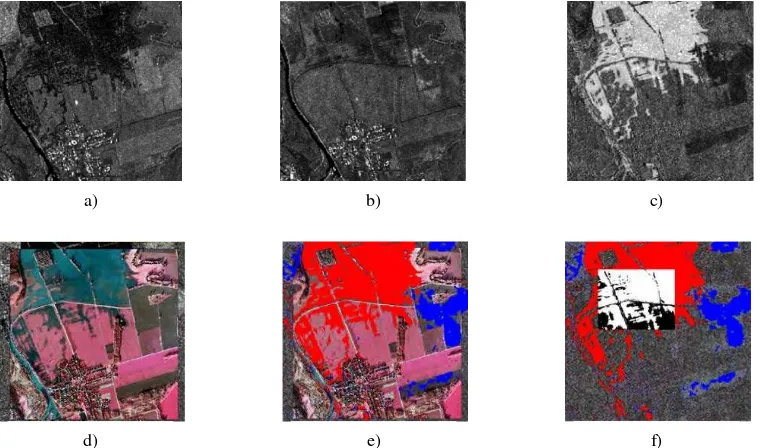
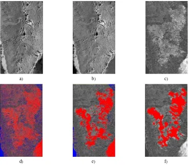
Another two HH-polarized TerraSAR-X ScanSAR scenes were acquired on 17/01/2011 and 08/02/2011 for the flood event of January 2011 at River Saale near Halle, Germany. A subset region and its classification result are visualized in figure 2. A co-registered RGB aerial image recorded on 17/01/2011 with a resolution of 0.5 m is used to generate a binary mask by the ISODATA segmentation algorithm using the software ERDAS Imagine. Another subset region is shown in figure 3. In this area strong backscattering occurs due to double bounce effects on partially submerged vegetation (figure 3a). It is very clear to observe three classes in this case.
The forest fire on La Palma in July/August 2009 is the last study case, for which a pair of HH-polarized TerraSAR-X scenes was acquired on 13/12/2007 and 09/08/2009. The original SAR data and its classification result are visualized in figure 4 and compared with the result derived by a
semi-automated object-based algorithm of Bernhard et al. (2011) implemented in the eCognition Developer software.
3.2 Results and Discussion
The classification results based on the hypothesis test shown in figure 1d and 4d are reasonable compared with their corresponding ratio images in figure 1c and 4c. However, overestimations of the changes occur and the results are noisy.
The classification results in figure 1e and 4e are post-processed by the graph-cut algorithm. They offer a significant improvement compared with the results only from the hypothesis test. In figure 4f a similar mask derived by a semi-automated object-based algorithm of Bernhard et al. (2011) implemented in the eCognition Developer software is shown. These two results are consistent and only differ in small details around the boundaries of the changed regions. The eCognition Developer software removes most of the scattered regions but overfits the shape of the boundary, whereas the graph-cut algorithm eliminates many scattered regions and holes but provides more reasonable estimation of the boundary.
In figure 2f the classification mask of the proposed method is compared with the binary mask generated by the ISODATA segmentation algorithm using the software ERDAS Imagine. The result of the comparison shows an overall accuracy of ~92.3% for this subset region. The difference of classification between the SAR and the aerial image is mostly located on the road and street areas. Because SAR is a side-looking sensor, the trees on the both sides of the road can disturb the observation by SAR sensor. In figure 2b many thin lines are displayed as dark pixels while no flood occurs. These areas are marked as no-changed area in figure 2e. This difference is mostly not related to the algorithm but the measuring principle of the SAR sensor.
It is interesting to observe three classes within one test area in figure 3. For a flood event negative changed areas are usually interpreted as flood. This interpretation is yet not true for figure 3 since most parts of figure 3b are non-water areas. This negative change is caused by the double/multiple bounce effect of partially flooded vegetation in figure 3a. If the flood water is not above the total vegetation, the water surface and lower sections of vegetation form a corner reflector and result in a strong signal return (Richards et al., 1987). The proposed method provides an effective algorithm to extract double/multiple bounced areas within a flood region.
4. CONCLUSION AND OUTLOOK
In this study we present a method consisting of a hypothesis test and graph-cut post-classification to detect significant three-class changes from two co-registered radiometrically calibrated SAR images. The concept of hypothesis test by Touzi et al. (1988) and Oliver et al. (1996) is rewritten by the incomplete beta function and adapted to the three-class classification problem. The initial classification by the hypothesis test is refined using the graph-cut algorithm proposed by Kolmogorov et al. (2004) and Boykov et al. (2004).
makes appropriate corrections. The post-processing by the graph-cut algorithm demonstrates an obvious improvement compared with the coarse classification by the hypothesis test. There is also a high correlation between the results obtained by the semi-automated object-based algorithm of Bernhard et al. (2011) and the graph-cut algorithm.
The remaining problem for change detection is the ambiguous interpretation of the detected changes. Further study will concentrate on the integration of textual information, auxiliary data and other biophysical models to support the interpretation of different detected changes.
REFERENCES
Bazi, Y., Bruzzone, L. and Melgani, F., 2005. An unsupervised approach based on the generalized gaussian model to automatic change detection in multitemporal sar images. IEEE Trans. Geoscience and Remote Sensing, 43(4), pp. 874–887.
Bernhard, E., Twele, A., and Gähler, M., 2011. Report on the ISPRS Workshop 2011, “Synergistic use of optical and radar data for rapid mapping of forest fires in the European Mediterranean”, Hannover, Deutschland.
Besag, J., 1986. On the statistical analysis of dirty pictures. Journal of the Royal Statistical Society. Series B, pp. 259–302.
Boykov, Y., Veksler, O., Zabih, R., 2011. Fast approximate energy minimization via graph cuts. IEEE Trans. Pattern Analysis and Machine Intelligence, 23(11), pp. 1222–1239.
Boykov, Y. and Kolmogorov, V., 2004. An experimental comparison of min-cut/ max-flow algorithms for energy minimization in vision. IEEE Trans. Pattern Analysis and Machine Intelligence, 26(9), pp. 1124-1137.
Ford, L. R. and Fulkerson, D. R., 1956. Maximal flow through a network. Canadian Journal of Mathematics, 8(3), pp. 399-404.
Geman, S. and Geman, D., 1984. Stochastic Relaxation, Gibbs Distributions, and the Bayesian Restoration of Images. IEEE Trans. Pattern Analysis and Machine Intelligence, 6, pp. 721-741.
Kolmogorov, V. and Zabin, R., 2004. What energy functions can be minimized via graph cuts? IEEE Trans. Pattern Analysis and Machine Intelligence, 26(2), pp. 147-159.
Li, S. Z., 1995. Markov random field modeling in computer vision. Springer-Verlag New York, Inc.
Lindgren, B., 1993. Statistical Theory. Chapman and Hall/CRC Texts in Statistical Science Series, Chapman & Hall.
Lu, D., Mausel, P., Brondizio, E. and Moran, E., 2004. Change detection techniques. International journal of remote sensing, 25(12), pp. 2365-2401.
Moser, G. and Serpico, S. B., 2006. Generalized minimum-error thresholding for unsupervised change detection from sar amplitude imagery. IEEE Trans. Geoscience and Remote Sensing, 44(10), pp. 2972-2982.
Oliver, C. and Shaun, Q., 2004. Understanding Synthetic Aperture Radar Images. SciTech Publishing.
Pearson, K., 1968. Tables of Incomplete Beta Functions, 2nd ed. Cambridge, England: Cambridge University Press.
Radke, R. J., Andra, S., Al-Kofahi, O. and Roysam, B., 2005. Image change detection algorithms: a systematic survey. IEEE Trans. Image Processing, 14(3), pp. 294-307.
Richards, J., Woodgate, P. and Skidmore, A., 1987. An explanation of enhanced radar backscattering from flooded forests. International Journal of Remote Sensing, 8(7), pp. 1093–1100.
Figure 1: Study area of Queensland, Australia. Subsets of TerraSAR-X amplitude data (© DLR 2013) of a) 05/01/2011 and b) 21/01/2011, c) intensity ratio image between b) and a), d) classification based on the hypothesis test, e) classification based on the hypothesis test and the graph-cut algorithm. In d) and e) positive- and negative-change are shown in red and blue colors, no-change is transparent.
Figure 2: Study area of Halle, Germany. Subsets of TerraSAR-X amplitude data (© DLR 2013) of a) 17/01/2011 and b) 08/02/2011, c) intensity ratio image between b) and a), d) co-registered aerial RGB image data, e) classification based on the hypothesis test and the graph-cut algorithm, g) classification with the binary mask derived from d). In e) and f) positive- and negative-change are shown in red and blue colors, no-change is transparent.
Figure 3: Study area of Halle, Germany. Subsets of TerraSAR-X amplitude data (© DLR 2013) of a) 17/01/2011 and b) 08/02/2011, c) intensity ratio image between b) and a), d) classification based on the hypothesis test and the graph-cut algorithm, positive- and negative-change are shown in red and blue colors, no-change is transparent.
a) b) c) d) e)
a) b) c)
d) e) f)
Figure 4: Study area of La Palma, Spain. Subsets of TerraSAR-X amplitude data (© DLR 2013) of a) 13/12/2007 and b) 09/08/2009, c) intensity ratio image between b) and a), d) classification based on the hypothesis test, e) classification based on the hypothesis test and the graph-cut algorithm, f) classification by Bernhard et al. (2011). In d), e) and f) positive and negative changes are shown in red and blue colors, no-change is transparent.
a) b) c)