IMPROVEMENT OF 3D MONTE CARLO LOCALIZATION
USING A DEPTH CAMERA AND TERRESTRIAL LASER SCANNER
S. Kanai a,*, R. Hatakeyama a, H. Date a
a Graduate School of Information Science and Technology, Hokkaido University, Kita-ku, Sapporo 060-0814, Japan - {kanai, hdate}@ssi.ist.hokudai.ac.jp, [email protected]
Commission IV/WG7 & V/4
KEY WORDS: Monte Carlo Localization, Depth Camera, Terrestrial Laser Scanner, GPGPU, IMU, Scene Simulation
ABSTRACT:
Effective and accurate localization method in three-dimensional indoor environments is a key requirement for indoor navigation and lifelong robotic assistance. So far, Monte Carlo Localization (MCL) has given one of the promising solutions for the indoor localization methods. Previous work of MCL has been mostly limited to 2D motion estimation in a planar map, and a few 3D MCL approaches have been recently proposed. However, their localization accuracy and efficiency still remain at an unsatisfactory level (a few hundreds millimetre error at up to a few FPS) or is not fully verified with the precise ground truth. Therefore, the purpose of this study is to improve an accuracy and efficiency of 6DOF motion estimation in 3D MCL for indoor localization. Firstly, a terrestrial laser scanner is used for creating a precise 3D mesh model as an environment map, and a professional-level depth camera is installed as an outer sensor. GPU scene simulation is also introduced to upgrade the speed of prediction phase in MCL. Moreover, for further improvement, GPGPU programming is implemented to realize further speed up of the likelihood estimation phase, and anisotropic particle propagation is introduced into MCL based on the observations from an inertia sensor. Improvements in the localization accuracy and efficiency are verified by the comparison with a previous MCL method. As a result, it was confirmed that GPGPU-based algorithm was effective in increasing the computational efficiency to 10-50 FPS when the number of particles remain below a few hundreds. On the other hand, inertia sensor-based algorithm reduced the localization error to a median of 47mm even with less number of particles. The results showed that our proposed 3D MCL method outperforms the previous one in accuracy and efficiency.
1. INTRODUCTION
With recent interest in indoor navigation and lifelong robotic assistance for human life support, there is an increased need for more effective and accurate localization method in three dimensional indoor environments. The localization is the ability to determine the robot’s position and orientation in the environment. So far, three typical methods have been proposed for the indoor localization; (1) based only on internal sensors such as an odometry or an inertial navigation, (2) utilizing observations of the environment from outer sensors in an a priori or previously learned map such as Monte Carlo Localization (MCL), and (3) relying on infrastructures previously-installed in the environments such as distinct landmarks such as bar-codes, WiFi access points or surveillance camera networks (Borenstein et al., 1997).
Among them, MCL gives one of the promising solutions for the localization when previously created environment map is available and the system installation should be realized at a low cost. The MCL is a kind of probabilistic state estimation methods (Thrun et al., 2005) which can provide a comprehensive and real-time solution to the localization problem. However, previous work of MCL has been mostly limited to 2D motion estimation in a planar map using 2D laser scanners (Dellaert et al., 1999; Thrun et al., 2001). Recently, a few 3D MCL approaches have been proposed where rough 3D models and consumer-level depth cameras are used as the environment maps and outer sensors (Fallon et al., 2012;
Hornung et al., 2014; Jeong et al., 2013). However, their localization accuracy and efficiency still remain at an unsatisfactory level (a few hundreds millimetre error at up to a few FPS) (Fallon et al., 2012; Hornung et al., 2014), or the accuracy is not fully verified using the precise ground truth (Jeong et al., 2013).
Therefore, the purpose of this study is to improve an accuracy and efficiency of 6DOF motion estimation in 3D Monte Carlo Localization (MCL) for indoor localization. To this end, firstly, a terrestrial laser scanner is used for creating a precise 3D mesh model as an environment map, and a professional-level depth camera is installed in the system as an outer sensor. GPU scene simulation is also introduced to upgrade the speed of prediction phase in MCL. Moreover, GPGPU programming is implemented to realize further speed up of the likelihood estimation phase, and anisotropic particle propagation is introduced based on the observations from an inertia sensor in MCL. The improvements in the localization accuracy and efficiency are verified by the comparison with a previous 3D MCL method (Fallon et al., 2012).
2. 3D MONTE CARLO LOCALIZATION
Monte Carlo Localization (MCL) is one of probabilistic state estimation methods (Thrun et al., 2005) using observation from outer sensor. The position and orientation of a system to be estimated is expressed by a state variable. A probability density function of the state variables is represented approximately by a finite set of “particles” each of which expresses a discrete instance of the state variables, and a progress of the probability
*Corresponding author:
Satoshi Kanai ( [email protected] )
distribution is estimated by repeating propagation, likelihood evaluation and weighting based on the observation, and resampling of the particles.
The 3D MCL algorithms of our study are extensions of the previous 3D MCL approach which made use of GPU scene simulation (Fallon et al., 2012). As our extensions, in order to increase the accuracy of a map and an outer sensor, a terrestrial laser scanner is introduced for creating a precise 3D mesh model as an environment map, and a professional-level depth camera is installed as an outer sensor. Moreover, in our second extensions, a GPGPU programming is implemented to realize a speed up of the localization process, and an anisotropic particle propagation based on the observations from an inertia sensor is introduced in order to increase the localization accuracy. Figure 1 shows a flow of our baseline 3D MCL algorithm. The state variable ��= [ �, �, �, ��, ��, ��] denotes a 6-DOF pose of each distribution respectively.
The depth camera pose �� can be estimated by the following steps;
1) Initialization: An initial filter distribution �| at � =0 is
created by assigning a same state �| into all of the particles in the distribution as Eq(3).
�| = {�| , �| , … . . . , � | }
2) Propagation: A predicted distribution ��+ |� of the next
time step � + is generated from a current filtered distribution ��|� by applying a system model of 6-DOF motion of the depth camera. In the baseline algorithm, the system model is given by a Gaussian noise model as Eq(4).
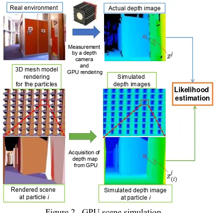
��+ |�= ��|�+ ℵ(�, ��) mesh model of an environment map. Each simulated depth image �� is easily obtained by GPU rendering whose viewpoint coincides with a camera pose expressed by an i-th particle ��+ |�∈ ��+ |� in the predicted distribution. In this study, an OpenGL function glReadPixels() is used to quickly obtain an two-dimennsional array of normalized depth values of �� from a depth buffer of GPU in one go. the simulated image �� corresponding to an i-th particle,
Figure 2. GPU scene simulation Figure 1. Our 3D MCL baseline algorithm
Particle
and is the number of pixels in a depth image. �̃ � and
�̃ are the maximum and minimum likelihood values respectivelyamong elements of a set {�̃ } each of which is evaluated by Eq(5) corresponding to an i-th particle. Using Eq(6), a normalized likelihood value � ∈ [ , ] for an i-th particle can be obtained.
used for the resampling.
By repeating the above from step 2) to 5), the particle distribution can be updated according to the observation from the depth camera, and state estimation of the camera pose �� is sequentially updated. GPU rendering is introduced in step 2) for generating simulated depth images in real time.
3. EFFICIENCY IMPROVEMENT OF THE
LOCALIZAITON BASED ON GPGPU PROGRAMMING
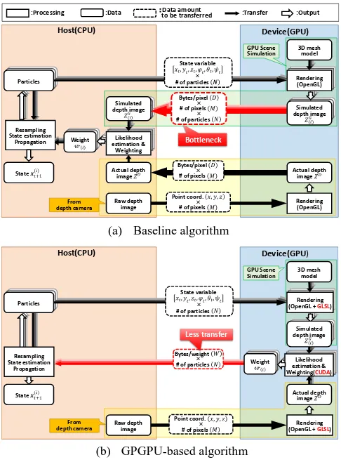
As shown in Figure 3-(a), in our baseline MCL algorithm described in section 2, processing other than GPU scene simulation (step 2)) are executed by CPU, and every simulated depth image �� which is rendered in GPU has to be uploaded directly to CPU right after the rendering using an OpenGL function glReadPixels().As a result, ( × × � byte data has to be uploaded in all from GPU to CPU in every time step, where N means the number of total particles, is the number of pixels in a depth image, and � is the number of bytes of one pixel data. In our setting, a professional-level depth camera (SR4000) is used, and it generates a depth image of 176×144 pixels in every frame. When a float-type variable (4 bytes) is used per pixel and 100 particles are included in a distribution, around 10Mbyte data has to be uploaded from GPU to CPU in every frame. Due to relatively slow execution speed of glReadPixels(), its transmission delay is not negligible, and it was observed that the delay caused a considerable bottleneck of the baseline MCL algorithm.
To reduce this delay, General Purpose computing on GPU (GPGPU) (Eberly, 2014) is introduced in the algorithm so that the GPU takes both GPU scene simulation (Step 2)) and likelihood estimation (Step 3)) as shown in Figure 3-(b). The
parallel processing of likelihood estimations for all particles can be handily implemented in GPGPU. In the GPGPU implementation, the simulated depth image �� is directly rendered using GLSL (OpenGL Shading Language). And using CUDA (Sanders et al., 2010), a resulting rendered image can be compared with the rendered actual depth image ��, and likelihood estimation and weighting can be processed on the GPU without transferring any simulated depth image data to the CPU. Finally, only a set of weights of the particles {� } only has to be transferred from GPU to CPU. Moreover, a likelihood value at a pixel in the right hand side of Eq.(5) can also be evaluated independently of the other pixel. So we parallelized this pixel-wise likelihood calculation using CUDA. As a result of this implementation, a set of weights {� } whose data amount is around × � byte (�: a number of bytes per one weight) in total only has to be uploaded from GPU to CPU per every frame. This can significantly reduce the data amount to be uploaded to about 400Byte. The effect of the implementation on our localization performance is explained in 5.2.
4. ACCURACY IMPROVEMENT OF THE
LOCALIZAITON WITH THE AID OF AN INERTIA SENSOR
As the other approach for the accuracy improvement in the localization, a small 6-DOF inertial measurement unit (IMU) is installed in the system. With the aid of this IMU, the
between the baseline and GPGPU-based algorithm
anisotropic particle propagation based on an actual observation from the IMU can be introduced in the propagation step (Step1)) in MCL.
Different from Gaussian-based isotropic particle propagation in the baseline MCL, more particles are allocated adaptively along the direction of the measured acceleration and angular acceleration given from the IMU. In the propagation step in the MCL, this anisotropic particle propagation is easily implemented by replacing the original propagation equation Eq(4) with Eq(10).
��+ = �� + ℵ(��, �̂�)
where, ��= [ ��, � �, ��, ���, ���, ��� ] is a 6D estimated
positional and rotational displacements derived from the numerical integration of the measured acceleration and angular acceleration of IMU at time step �. We also assume from the observation that a standard deviation of each displacement in the system model is comparable to the estimated displacement
��, and therefore set as �̂�= [ � � , � � , �� , ��� , ��� , ��� ].
5. EXPERIMENTS
5.1 Setup
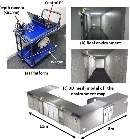
The improvement in efficiency and accuracy is verified in localization experiments in an indoor environment. Figure 4 shows our experimental setup. As shown in Figure 4-(a), a professional-level depth camera (SR4000, TOF camera, Pixel resolution: 176×144) and an IMU (ZMP IMU-Z Tiny Cube) were attached on a top surface of a small wagon. A laptop PC (Windows-7, Corei7-3.7GHz, and GeForce GT-650M) on the wagon recorded a time sequence both of raw depth image from the depth camera and acceleration data from the IMU on site. On the other hand, the localization calculation was done on the other desktop PC (Windows-7, Corei7-2.93GHz, and GeForce GTX-770).
As a preparation, 3D point clouds of corridor space (9× ×
. m) in a university building shown in Figure 4-(b) was first measured by a terrestrial laser scanner (FARO-Focus 3D), and a precise 3D mesh model with 141,899 triangles shown in Figure 4-(c) was created as an precise environmental map of the space using a commercial point cloud processing software. GeForce GTX-770 was used when investigating the effect of GPGPU programming on an efficiency of the localization.
5.2 Results
Efficiency improvement by GPGPU programming: Figure
5 compares the averaged processing time for single time step of MCL. 6-DOF depth camera pose is estimated in the experiment. From this figure, it is clearly shown that the proposed GPGPU-based algorithm is effective in reducing the time for localization when the number of particles remains below a few hundreds which is a general setting of this MCL.
However, the improvement in the processing speed was not so significant even when the GPGPU implementation is applied as shown in Figure 5. The reason for this behaviour is that GPGPU coding generally requires a sophisticated knowledge of parallel processing, and there is still a room for more efficient parallelization coding in likelihood estimation and weighting processing in GPU.
Accuracy improvement by IMU: Figure 6 compared the
estimated camera positions using the baseline and proposed IMU-based algorithm in case of 200 particles. In this
11m 8m
Depth camera (SR4000)
Wagon
Control PC
(a) Platform
(b) Real environment
(c) 3D mesh model of the environment map
Figure 4. The platform and the environment map
0 20 40 60 80 100 120 140 160 180 200
100 150 200 250 300 350 400 450 500
Av
e
ra
g
e
p
ro
ce
ss
in
g
t
im
e
[
m
se
c]
# of particles
手法 (GPGPUなし) 手法 (GPGPUあり)
Effective range when using GPGPU
Without GPGPU With GPGPU (GTX770)
Figure 5. Processing time with and without GPGPU
5m
6m
Ground Truth
推定位置
(
提案手法
)
推定位置
(
提案手法
)
Ground truth
Baseline algorithm
With IMU
Figure 6. The traces of estimated camera positions with and without IMU
experiment, 6-DOF depth camera pose was estimated, but the accuracy verification is verified only in a planer position [ , ] of 2-DOF. The ground truth trace of the wagon was precisely collected from physical marker recording attached under the wagon using a terrestrial laser scanner. The estimated positions with the aid of the IMU locate much closer to the ground truth than those without IMU.
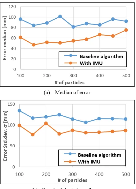
Figure 7 shows the median and standard deviation of localization errors in different settings of the number of particles. In all settings, the IMU-based algorithm outperformed the baseline one, and the averaged median of the localization errors from the ground truth was reduced by 34%. And as shown in Figure 8, no significant decrease in the performance was observed when introducing the IMU. Table 1 summarizes the performances between the proposed MCL method with IMU and the previous 3D MCL study (Fallon et al., 2012). The table shows that our MCL method realized much smaller localization error (16%) even with 57% less particles.
6. SUMMARY
Several methods were proposed to improve the accuracy and efficiency of 3D Monte Carlo Localization (MCL) for indoor localization. For the baseline algorithm, a terrestrial laser scanner was used for creating a precise 3D mesh model as an environment map, and a professional-level depth camera was installed as an outer sensor. Moreover, two original approaches were proposed for the improvement. As a result, it was confirmed that GPGPU-based algorithm was effective in increasing the computational efficiency to 10-50 FPS when the
number of particles remain below a few hundreds. On the other hand, inertia sensor-based algorithm reduced the localization error to a median of 47mm even with less number of particles. The results showed that our proposed 3D MCL method outperforms the previous one in accuracy and efficiency aspects.
References
Borenstein, J., Everett, H.R., Feng, L., and Wehe, D., 1997, Mobile robot positioning: Sensors and techniques. Journal of Robotic Systems, 14(4), pp.231–249.
Dellaert, F., Fox, D., Burgard, W., and Thrun, S., 1999. Monte Carlo Localization for mobile robots. IEEE International Conference on Robotics and Automation (ICRA), pp.1322– 1328.
Doucet, A, Freitas, N., and Gordon, N., 2001. Statistics Sequential Monte Carlo Methods in Practice, Springer, New York, pp.437-439.
Eberly, D.H., 2014. GPGPU Programming for Games and Science, CRC Press, Boca Raton.
Fallon, M.F., Johannsson, H., and Leonard, J.J., 2012. Efficient scene simulation for robust monte carlo localization using an RGB-D camera. IEEE International Conference on Robotics and Automation (ICRA), pp.1663–1670.
Hornung, A., Oswald S., Maier D., and Bennewitz, M., 2014. Monte carlo localization for humanoid robot navigation in complex indoor environments. International Journal of Humanoid Robotics, 11(2), pp. 1441002-1–1441002-27. Jeong, Y., Kurazume, R., Iwashita Y., and Hasegawa T., 2013, Global Localization for Mobile Ro bot using Large-scale 3D
(b) Standard deviation of error
Figure 7. Localization error in different particle settings
0
Figure 8. Processing time per frame in different particle settings
0
100 150 200 250 300 350 400 450 500
処理時間
Table 1. Comparison of the performances between the proposed method and [Fallon et al., 2012]
Environmental Map and RGB-D Camera. Journal of the Robotics Society of Japan, 31(9), pp.896–906.
Sanders, J., and Kandrot, E., 2010. CUDA by Example: An Introduction to General-Purpose GPU Programming, Addison-Wesley Professional, Boston.
Thrun, S., Fox, D., Burgard, W., and Dellaert, F., 2001. Robust Monte Carlo localization for mobile robots. Artificial Intelligence, 128(1), pp.99–141.
Thrun, S., Burgard, W., and Fox, D., 2005. Probabilistic Robotics, MIT Press, Cambridge, pp.189–276.