Estimation of solar radiation in Australia from rainfall and
temperature observations
D.L. Liu
∗, B.J. Scott
NSW Agriculture, Wagga Wagga Agricultural Institute, PMB, Wagga Wagga, NSW 2650, Australia Received 1 May 2000; received in revised form 9 June 2000; accepted 21 June 2000
Abstract
This study evaluated the accuracy of several models for estimating daily solar radiation (Q) across Australia. Data from 39 sites were taken from MetAccess. The sites were grouped into four climatic zones. Coefficients of nine models, including two newly developed formulae, were fitted for the 39 sites. Correlation coefficients (R2) between estimated Q and measured Q and root mean squared error (RMSE) associated with the estimates were calculated. It was concluded that models which expressed rainfall as a binary quantity (1 for rainfall>0; 0 for rainfall=0) performed better than those using amount of rainfall (precipitation in mm). The best performed models, one using temperature data only, one using rainfall data only and one using rainfall and temperature were further evaluated. A newly developed model that included temperatures (minimum and maximum) and rain-day information proved the best method. Using the coefficients for estimates of Q at the same sites, averaged R2was 0.68, 0.74 and 0.79 and RMSE was 3.24, 3.05 and 2.89 MJ m−2, for the model using rainfall only, temperature only and both rainfall and temperature, respectively. When Q was estimated using the coefficients from other sites, estimation of Q within eastern and southern zones were more reliable than in northern and central zones.
In general, the model using both temperature and rainfall was the best model for either estimated Q for the site where coefficients of the model were developed at the site or imported from other sites. However, in some tropical coastal sites of Australia, such as Broome and Darwin, estimates of Q based on rainfall only can be more reliable when the coefficients were imported from other sites. It was concluded that radiation within a similar climatic region could be well estimated with no local recording, regardless of distance between sites. © 2001 Elsevier Science B.V. All rights reserved.
Keywords: Solar radiation; Precipitation; Overcast conditions; Air temperature; Atmospheric transmittance
1. Introduction
Daily radiation is required by most models that sim-ulate crop growth because growth is primarily based on the photosynthetic processes which involve the utilisation of radiation and its conversion to chemi-cal energy. However, solar radiation is an infrequently measured meteorological variable, compared to tem-perature and rainfall. In Australia, the meteorological
∗Corresponding author.
E-mail address: [email protected] (D.L. Liu).
database MetAccess (Donnelly et al., 1997) contains 16,000 weather stations, nearly all of which have daily rainfall records while 1,400 stations have records of temperature. Only 50 stations have records of solar ra-diation. Lack of solar radiation data is also common in other countries, such as USA (Richardson, 1985; Hook and McClendon, 1992) and Canada (De Jong and Stewart, 1993), and can be a major limitation to the use of crop growth simulation models.
In order to use crop simulation models, techniques are required to estimate radiation based on other com-monly measured meteorological variables for the days
or years when the data are missing, or for the sites when the data are not measured. Two methods used to generate radiation data are stochastic generation (Nicks and Harp, 1980; Richardson, 1981; Richard-son and Wright, 1984) and empirical relationships (Bristow and Campbell, 1984; McCaskill, 1990a,b; Hook and McClendon, 1992; De Jong and Stewart, 1993; Hunt et al., 1998).
An example of stochastic weather generation is the method using a continuous multivariate stochastic process to generate weather data including radiation (Richardson, 1981; Richardson and Wright, 1984). Sharpley and Williams (1990a,b) adopted this ap-proach to generate radiation data using only the monthly means of daily radiation as inputs.
Stochastic generated data may be useful to explore possible model scenarios for an average theoretical situation of long term simulation. However, the data generated by this approach cannot be used for model validation and simulation analysis for a particular period of time as the method may not generate the data to match the actual weather at a particular time of interest. It fails to generate weather extremes reli-ably, such as frost that can damage crops (Wallis and Griffiths, 1995).
Using empirical relationships requires the devel-opment of a set of equations to estimate solar radia-tion from the commonly measured meteorological variables. A number of formulae and methods have been reported using this approach (Fitzpatrick and Nix, 1970; Bristow and Campbell, 1984; Richardson, 1985; Hook and McClendon, 1992; De Jong and Stewart, 1993). Daily total extraterrestrial radiation (Qo) is often included in the relationships. The
under-lying approach is to express solar radiation reaching the earth surface (Q) as a fraction of Qo. This is based
on the attenuation of incoming radiation through the atmosphere. The physics involved in the interac-tion between radiainterac-tion and atmospheric constituents are complex, but the relationship between the atmo-spheric transmittance and some weather variables can be empirically described. Parameters used as inputs in the relationships include sunshine duration (Hux-ley, 1973; Schulze, 1976; Boisvert et al., 1990), mean humidity (Fitzpatrick and Nix, 1970), temperature (Richardson, 1985), rainfall (McCaskill, 1990a,b), or in combination (Hook and McClendon, 1992). Hayhoe (1998) recently evaluated the empirical
ap-proaches for estimating solar radiation and compared them to stochastic weather generation (Sharpley and Williams, 1990a,b). He found that an empirical model based on temperature and rainfall provided better estimates than the stochastic model.
Availability of weather data at locations varies from only one variable to several variables, so models de-veloped should suit the varying availability of data. The aim of this study was to evaluate the accuracy and applicability of several models for estimating daily value of solar radiation (Q) across Australia for differ-ent situations: only rainfall available, only temperature available, or both rainfall and temperature available at a site with or without some radiation recordings.
2. Materials and methods
2.1. Data collection
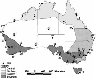
Fig. 1 shows the location of stations used and broad climatic regions of Australia. The northern zone is the summer rainfall tropical; eastern zone contains summer rainfall subtropical and uniform rainfall tem-perate; southern zone contains winter rainfall temper-ate; the central zone is the arid subtropical and arid temperate (Australian Bureau of Meteorology, 1997). Table 1 lists the details of 39 sites with radiation data, which were obtained from MetAccess (Donnelly et al., 1997) for this study. These sites have daily records in the database with 4 years or more of min-imum temperature, maxmin-imum temperature, rainfall and solar radiation. Records for temperature and radi-ation relate to the 24 h starting at 09.00 h on the day of interest. The data records of rainfall relate to the 24 h up to 09.00 h on the day of interest. Although the amount of rainfall recorded at this time most likely fell in the previous day, no displacement was done as the manner of the records is the convention of the meteorological data inputs by Australian Bureau of Meteorology (Donnelly et al., 1997). Thus, it should be noted that if the coefficients of models reported in this study are applied to data records in the different way, appropriate displacement must be taken.
Fig. 1. Sites with historical recordings of radiation, rainfall and temperatures and geographic and climatic regimes of Australia. The site number is referenced in Table 1.
3 years data were used for the regression; otherwise 5 years data were used. The years with no missing data were selected first. If the number of years with no missing data was insufficient, the years with fewer missing data were selected. The second file contained the remaining data that were used for validation of the model at the same site. The third file contained all data and was used for validations of the predictability of the site using coefficients obtained from other sites.
Daily total extraterrestrial radiation (Qo) was
cal-culated as a function of latitude, day of year, solar angle and solar constant, using the method of Duffie and Beckman (1980). This method included the rela-tive distance of earth from the sun. Some authors (e.g. Bristow and Campbell, 1984) did not include this term as it varies<3.5% from unity.
2.2. Equations
2.2.1. Estimation of solar radiation using temperature only
Bristow and Campbell (1984) developed a model for estimation of solar radiation reaching the earth’s
surface (Q), based on the fraction of daily total at-mospheric transmittance of the extra-terrestrial solar radiation, which is determined by the range of daily air temperature extremes (D) as
Q=Qoa(1−exp(−bDc)) (1)
where a, b and c are empirical coefficients, determined for the particular sites from measured solar radiation data. D is the diurnal range of air temperature and is calculated as
D=Tmax−
Tmin(j )+Tmin(j+1)
2
where Tmax is the daily maximum temperature (◦C),
Tmin(j) andTmin(j +1)the daily minimum
Table 1
Details of the stations and records used in this study Site no. Site name Operating
authority
1 Broome AMOa 17.95 122.22 7 10 544 1986–1992
2 Cloncurry JTTREb 20.40 140.50 189 700 291 1978–1981
3 Cowley JTTRE 17.67 146.12 4 20 2274 1978–1981
4 Darwin AP AMOc 12.42 130.87 31 10 1695 1976–1992
5 Halls Creek AMO 18.23 127.65 422 376 528 1969–1991
6 Innisfail DPId 17.32 145.97 40 30 3500 1978–1981
7 Rockhampton AMO 23.37 150.29 10 20 832 1973–1988
8 Townsville AMO 19.25 146.75 8 15 1100 1971–1991
Eastern
9 Brisbane AMO 27.37 153.12 4 20 1188 1983–1992
10 Canberra AMO 35.30 149.18 571 102 632 1983–1992
11 Condobolin ARS 33.05 147.23 195 315 469 1978–1987
12 Hobart AP AMO 42.82 147.50 4 10 510 1967–1992
13 Melbourne AMO 37.80 144.95 35 10 660 1976–1986
14 Nambour DPI 26.63 152.93 25 10 1731 1973–1980
15 Orange ARSe 33.30 149.07 922 193 946 1977–1987
16 Sydney AMO 33.93 151.17 6 10 1104 1983–1992
17 Williamtown AMO 32.78 151.82 9 10 993 1968–1988
Southern
18 Adelaide AP AMO 34.95 138.53 6 10 450 1983–1992
19 Albany AMO 34.95 117.80 68 10 789 1970–1988
20 Esperance AMO 33.82 121.20 25 5 615 1987–1991
21 Geraldton AMO 28.78 114.68 33 5 459 1968–1988
22 Glen Osmond WI 34.97 138.62 122 10 609 1969–1986
23 Hamilton RSf 37.82 142.05 200 92 702 1974–1988
24 Kyabram RIg 36.32 145.05 104 183 464 1975–1992
25 Laverton AMO 37.85 144.75 18 10 560 1968–1992
26 Mildura AP AMO 34.23 142.07 50 295 296 1969–1992
27 Perth AMO 31.58 115.97 20 15 801 1973–1992
28 Wagga Wagga AMO 35.17 147.43 212 295 558 1968–1990
29 Wundowie CSIROh 31.77 116.48 330 150 596 1978–1981
Central
30 Alice Spring AMO 23.78 133.87 546 895 272 1968–1992
31 Carnarvon AMO 24.87 113.65 4 10 227 1986–1992
32 Forrest AMO 30.83 128.12 156 102 179 1968–1992
33 Kalgoorlie AMO 30.77 121.43 365 315 265 1975–1992
34 Learmonth AMO 22.23 114.08 5 10 240 1968–1992
35 Longreach AMO 23.42 144.28 192 529 427 1968–1991
36 Meekatharra AMO 26.62 118.55 517 417 209 1986–1992
37 Oodnadatta AP AMO 27.58 135.43 113 508 170 1969–1985
38 Port Hedland AMO 20.37 118.62 9 3 298 1968–1991
39 Woomera AMO 31.13 136.48 165 193 191 1968–1988
aAMO: Australian Meteorological Officer. bJTTRE: Joint Trial Tropic Research Establishment. cAP: Airport.
dDPI: Department of Primary Industry. eARS: Agricultural Research Station. fRS: Research Station.
gRI: Research Institute.
the method for estimating radiation in the case when rainfall data are not available.
Two other models estimating solar radiation from temperature data were Eq. (2) (Richardson, 1985) and Eq. (3) (Hargreaves et al., 1985):
Q=Qoa(Tmax−Tmin)b (2)
Q=Qoa p
Tmax−Tmin+b (3)
where a, b are the coefficients.
2.2.2. Estimation of solar radiation using rainfall only
McCaskill (1990a) reported a method using Fourier series with incorporated rain-day information as
Q =a+bcos(θ )+csin(θ )+dcos(2θ )
+esin(2θ )+fRj−1+gRj+hRj+1 (4)
whereθ is the day of the year converted to radian, R the transformed rainfall data and its subscriptsj −1,
j and j +1 refer to the previous, current and next days, and a, b, c, d, e, f, g and h are the coefficients determined by regression. The transformation used to calculate R (rainfall) data was to encode rain-days: if P >0,R =1;P =0,R =0, where P is precipita-tion. The performance of Eq. (4) (Meinke et al., 1995) was considered to be similar to the WGEN stochastic weather generator (Richardson, 1981; Richardson and Wright, 1984).
Eq. (4) does not include Qo, but the site-specific
coefficients (a, b, c, d and e) with the functions of Fourier series will empirically describe the seasonal changes of radiation at the site where the data were collected. In another report, McCaskill (1990b) related
Q to Qoand rain-day information as
Q=aQo+bRj−1+cRj+dRj+1 (5)
where a, b, c and d are coefficients determined by re-gression and R is as defined in Eq. (4). The coeffi-cient a is the atmospheric transmittance with no rain-fall recorded on the day, the day before or the day after, while b, c, and d are the amounts of radiation reduction (MJ m−2) when it rained on the day before, on the day and on the day after, respectively.
2.2.3. Estimation of solar radiation using both temperature and rainfall
De Jong and Stewart (1993) used precipitation and the range of daily temperature extremes for estimation of solar radiation as
Q=aQoDb(1+cP+dP2) (6)
where P is the total precipitation (mm) on the day, D is defined as in Eq. (1). Hayhoe (1998) demonstrated that Eq. (6) provided better estimates of radiation than WXGEN (Sharpley and Williams, 1990a,b). Eq. (6) expressed the effect of precipitation on radiation as multiplicative. Hunt et al. (1998) developed Eq. (7) to include the effect of P as an additive formula:
Q=aQo p
Tmax−Tmin+bTmax+cP+dP2+e (7)
where a, b, c, d, e are the coefficients.
By analysing various forms with both temperature and rainfall variables across Australia, we propose two equations in the form of
Q=Qoa(1−exp(−bDc))(1+dRj−1
+eRj+fRj+1)+g (8)
Q=Qoa(1−exp(−bDc))+dRj−1
+eRj+fRj+1+g (9)
where a, b, c, d, e, f, and g are the coefficients, and D and R are as defined in Eqs. (1) and (4), respectively. The expression for the three rainfall is consistent with McCaskill (1990a,b).
In Eq. (1), the constant a is the maximum clear sky atmospheric transmittance (ξmx) which is defined as
the ratio of Q to Qowhen D is very large. In Eq. (8), ξmxat the given site can be approximated by ξmx=a+
g Qo
which indicates that wheng =0.0, ξmx =a; when g 6= 0, ξmx is a function of Qo. Hence, ξmx varies
with season. When g > 0, ξmx is larger in winter
2.3. Data analysis
The SHAZAM software was used for non-linear least squares regression (White, 1997). Regression residuals in some sites had a seasonal pattern, when expressed as the difference between observed Q and calculated Q. In order to overcome the seasonal het-erogeneity of error, all equations, except Eq. (4), were divided by Qo for the procedure of regression
analysis. To ensure stability of the coefficients, a range of initial values for the regressions was used to run the program. The coefficients of models were validated using the second set of data for the same station, or using the third set data (all data) for other sites. Goodness of fit for validations was assessed by squared correlation coefficients (R2) between the es-timated Q and recorded Q and the root mean square error (RMSE) associated with the estimation.
3. Results and discussion
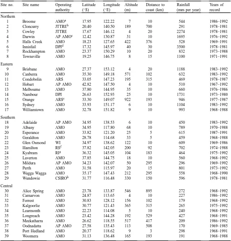
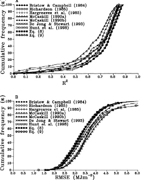
The performances of the nine models (Eqs. (1)–(9)) for regression of coefficients were compared in Fig. 2. Among the three models using temperature data only (Eqs. (1)–(3)), Eq. (1) (Bristow and Campbell, 1984) had highest values in R2 and lowest RMSE. Eq. (2) (Richardson, 1985) was more accurate than Eq. (3) (Hargreaves et al., 1985). Models using rainfall only (Eqs. (4) and (5)) had similar R2and RMSE. Among the four models which used both temperature and rain-fall data (Eqs. (6)–(9)), Eq. (8) had highest R2 and lowest RMSE, while Eq. (7) was the worst. Compared between approaches, Eqs. (8) and (9) which expressed rainfall as a binary quantity, were superior to Eqs. (6) and (7) which used the amount of rainfall, as the cu-mulative frequency (CF) showed.
In the Fig. 2, the low value tail of CF contained values ofR2 <0.4, which resulted from Darwin by Eqs. (1)–(6) and Broome by Eqs. (3) and (7). The low-est R2by Eqs. (8) and (9) were also Darwin (R2=0.5) and Broome (R2=0.6). This suggested Darwin and Broome were the most difficult sites to be estimated among the 39 sites. The CF distribution shows the es-timates of solar radiation using rainfall only (Eqs. (4) and (5)) had generally worse performance than the models involving temperature, indicating rainfall
ac-counted for less variation in daily radiation than tem-perature.
In general, for empirical equations such as those presented here, the more variables an equation has, the higher chance the model gets a better fit of observed data. However, estimates of radiation using Eqs. (6) and (7), which included both temperature and precipi-tation data, were worse than Eq. (1), which used tem-perature data only. This suggests that precipitation, as expressed in Eqs. (6) and (7) in mm, does not ade-quately account for the variance in the observed ra-diations. The better performance of Eqs. (8) and (9) suggested that the approach using rainfall as a binary quantity (1 for rain, 0 for no rain) was better than the approach using daily rainfall involved in a model for estimates of radiation in Australia. However, Eqs. (8) and (9) have more coefficients than other equations except Eq. (5).
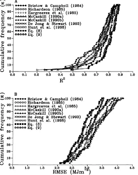
Fig. 3 shows the validations of these models at the 39 locations across Australia. The models that pro-duced a low R2 for the sites of Darwin and Broome also had a low R2 for the validation in the respective sites. Similar to the performance in the parameteris-ing stage, Eq. (8) provided the best estimates of radia-tion with largest R2and smallest RMSE values in CF
functions. This suggests that if temperature and rain-fall data are available, Eq. (8) should be used and can provide a good method for estimates of radiation with greater accuracy than other methods.
The estimates of Q using the coefficients derived from the same site required some recorded solar ra-diation data, but in many cases even a short period record of radiation was not available. To resolve this difficulty we investigated the possibility of using co-efficients developed at other similar sites.
Fig. 2. Comparison of cumulative frequency (CF) of (A) squared correlation coefficients (R2) and (B) the root mean square error (RMSE) between nine models during the calibration phase across all sites.
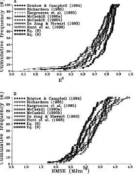
as they had lower R2and higher RMSE distributions, while Eq. (8) was ranked the best. It should be noted that Eqs. (4) and (5) showed a similar distribution in CF functions for the regression (Fig. 2) and validations (Fig. 3). However, Eq. (5) was superior to Eq. (4) when the coefficients were used for other sites (Fig. 4). This is because Eq. (4) used coefficients of Fourier series, which did not include latitude. Thus, there is no basis to apply the coefficients to sites other than that where the model was parameterised.
Therefore, Eqs. (1), (5) and (8) were selected to rep-resent the methods of estimating radiation when only temperature is available, when only rainfall is
able and when both temperature and rainfall are avail-able, respectively. Tables 2–4 showed the coefficients for Eqs. (1), (5) and (8), respectively. The regression coefficients within each climatic region showed little variation.
coeffi-Fig. 3. Comparison of cumulative frequency (CF) of (A) squared correlation coefficients (R2) and (B) the root mean square error (RMSE) between nine models during the independent testing phase across all sites.
cient a in Australia were similar to the range between 0.72 and 0.77 estimated in USA (Bristow and Camp-bell, 1984). The coefficient a in Eq. (5) was the total atmospheric transmittance on dry days. Mean value of
a varied little between regions. The value of 0.65 for a
in the northern regions was very close to the value of 0.66 reported by McCaskill (1990b) for northern Aus-tralia including the tropics and eastern regions. Three rain-days reduced solar radiation in the middle day by 9.4, 7.2, 6.6 and 8.2 MJ m−2in northern, eastern, southern and central regions, respectively. This com-pared with 8.6 MJ m−2 in the northern Australia re-ported by McCaskill (1990b). In our studies, results showed a reduction of 1.2 MJ m−2 by the previous
Fig. 4. Comparison of cumulative frequency (CF) of (A) squared correlation coefficients (R2) and (B) the root mean square error (RMSE) between nine models using coefficients from one site for estimates of Q for the other 38 sites. Each CF curve was based on 1448 values.
The constant g in Eq. (8) varied from −6.48 to 4.86, which had 23 out of 39 sites within the range of ±1 (Table 4). This indicated there is small seasonal variation in atmospheric transmittance at the majority of sites in Australia. The five sites with g > 1, are all the inland sites with larger ξmxin winter than in
summer. The 11 sites withg <−1, which had a larger ξmx in summer than in winter, are all coastal sites,
except Condobolin (g= −1.65).
In Eq. (8), the reduction in solar radiation by rain-fall was expressed (1+dRj−1+eRj +dRj+1) as a
fraction (multiplicative), rather than absolute values (additive) (Eq. (9)). The results showed that formula of Eq. (8) expressed the rainfall effect better than
ad-ditive expression. A similar example was the com-parison between Eqs. (6) and (7), when the coeffi-cients are applied to other sites for estimating radia-tion, the additive effect of rainfall from one site can substantially overestimate or underestimate solar radi-ation from another site. Atwater and Ball (1981) com-puted cloud day radiation in proportion to the clear sky radiation, i.e. the multiplicative approach, while McCaskill (1990b) tested one version of a multiplica-tive formula of Eq. (5) which was a poorer fit than the additive formulae (Eq. (5)).
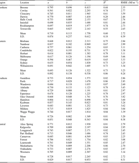
Table 2
Coefficients and statistics for estimation of solar radiation by Eq. (1) (Bristow and Campbell, 1984), using temperature data only
Region Location a b c R2 RMSE (MJ m−2)
Northern Broome 0.795 0.696 0.415 0.44 2.35
Cowley 0.561 0.022 2.293 0.74 2.77
Cloncurry 0.745 0.011 1.965 0.61 3.59
Darwin 0.770 0.087 1.410 0.28 2.46
Halls Creek 0.753 0.009 2.153 0.67 2.76
Innisfail 0.698 0.035 1.688 0.81 2.44
Rockhampton 0.697 0.019 1.977 0.74 2.73
Townsville 0.665 0.027 2.163 0.55 2.65
Mean 0.710 0.113 1.758 0.60 2.72
S.D. 0.074 0.237 0.612 0.18 0.39
Eastern Brisbane 0.668 0.012 2.313 0.75 2.84
Nambour 0.837 0.102 0.969 0.67 2.99
Canberra 0.757 0.061 1.254 0.83 3.11
Condobolin 0.822 0.193 0.731 0.75 3.38
Horbart 0.614 0.081 1.383 0.78 3.11
Melbourne 0.617 0.126 1.194 0.69 3.66
Orange 0.594 0.467 0.619 0.65 3.33
Sydney 0.635 0.054 1.830 0.73 3.25
Williamtown 0.691 0.042 1.605 0.73 3.34
Mean 0.693 0.126 1.322 0.73 3.23
S.D. 0.092 0.138 0.538 0.06 0.24
Southern Geraldton 0.733 0.054 1.573 0.82 2.86
Perth 0.717 0.028 1.670 0.86 2.83
Wundowie 0.684 0.118 1.035 0.87 2.60
Adelaide 0.730 0.133 1.123 0.78 3.43
Albany 0.729 0.088 1.191 0.81 2.97
Esperance 0.674 0.120 1.225 0.78 2.97
Glen Osmond 0.668 0.048 1.761 0.76 3.82
Hamilton 0.804 0.134 0.890 0.79 3.60
Kyabram 0.837 0.143 0.823 0.81 3.24
Laverton 0.683 0.081 1.252 0.73 3.62
Mildura 0.715 0.019 1.825 0.84 3.04
Wagga Wagga 0.744 0.017 1.814 0.84 3.39
Mean 0.726 0.082 1.349 0.81 3.20
S.D. 0.051 0.048 0.363 0.04 0.38
Central Alice Spring 0.771 0.012 1.930 0.81 2.79
Kalgoorlie 0.709 0.009 2.197 0.84 2.95
Longgreach 0.743 0.007 2.171 0.82 2.45
Part Hedland 0.713 0.046 1.686 0.74 2.43
Carnarvon 0.685 0.001 4.569 0.83 2.25
Forrest 0.706 0.021 1.754 0.82 3.08
Learmonth 0.761 0.049 1.551 0.85 2.47
Meekatharra 0.754 0.009 2.208 0.86 2.70
Oodnadatta 0.733 0.007 2.276 0.83 2.97
Woomera 0.705 0.009 2.307 0.82 3.14
Mean 0.728 0.017 2.265 0.82 2.72
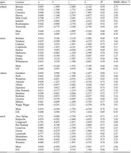
Table 3
Coefficients and statistics for estimation of solar radiation by Eq. (5) (McCaskill, 1990b), using rainfall data only
Region Location a b c d R2 RMSE (MJ m−2)
Northern Broome 0.695 −1.969 −3.068 −4.142 0.59 2.75
Cowley 0.554 −1.360 −1.753 −5.640 0.44 3.21
Cloncurry 0.668 −2.584 −2.815 −7.983 0.43 3.64
Darwin 0.698 −1.180 −2.793 −4.877 0.32 2.50
Halls Creek 0.704 −1.357 −3.681 −4.531 0.52 2.79
Innisfail 0.579 −0.463 −2.369 −4.612 0.54 3.01
Rockhampton 0.642 −0.060 −2.756 −5.420 0.52 3.47
Townsville 0.651 −0.775 −3.209 −4.756 0.49 3.03
Mean 0.649 −1.219 −2.805 −5.245 0.48 3.05
S.D. 0.056 0.809 0.573 1.206 0.08 0.38
Eastern Brisbane 0.614 0.146 −2.126 −3.982 0.60 3.59
Nambour 0.625 −0.299 −1.986 −4.272 0.53 3.64
Canberra 0.624 0.219 −1.891 −3.642 0.75 3.47
Condobolin 0.650 −1.615 −4.161 −0.795 0.80 3.11
Horbart 0.535 0.052 −0.504 −1.995 0.69 3.61
Melbourne 0.542 −0.064 −1.260 −2.999 0.70 3.56
Orange 0.543 −0.194 −1.921 −0.407 0.67 3.27
Sydney 0.610 0.124 −1.947 −3.913 0.64 3.96
Williamtown 0.631 0.338 −1.588 −4.061 0.59 4.18
Mean 0.597 −0.144 −1.932 −5.105 0.66 3.60
S.D. 0.044 0.587 0.976 1.204 0.08 0.32
Southern Geraldton 0.692 0.506 −1.740 −3.457 0.80 3.11
Perth 0.641 0.169 −1.858 −3.411 0.82 3.04
Wundowie 0.556 −0.651 −0.976 −2.565 0.83 2.70
Adelaide 0.638 −1.227 −3.147 −0.336 0.75 3.58
Albany 0.570 −0.937 −2.042 0.266 0.67 3.65
Esperance 0.610 0.012 −1.487 −2.643 0.74 3.43
Glen Osmond 0.611 −0.117 −1.219 −3.760 0.73 3.74
Hamilton 0.598 −0.041 −0.886 −2.537 0.72 3.77
Kyabram 0.634 −0.815 −3.018 −0.437 0.82 3.16
Laverton 0.573 −0.159 −0.985 −2.536 0.68 3.81
Mildura 0.641 −0.609 −1.498 −3.703 0.77 3.28
Wagga Wagga 0.656 −0.281 −2.222 −4.358 0.78 3.61
Mean 0.618 −0.346 −1.756 −4.554 0.76 3.41
S.D. 0.040 0.506 0.752 1.634 0.05 0.35
Central Alice Spring 0.721 −0.680 −3.766 −6.730 0.71 3.15
Kalgoorlie 0.674 −0.292 −2.444 −4.652 0.78 3.26
Longgreach 0.701 −0.455 −2.871 −5.838 0.72 2.80
Part Hedland 0.693 −0.748 −3.252 −5.009 0.73 2.64
Carnarvon 0.696 −0.273 −1.760 −3.773 0.83 2.41
Forrest 0.661 −0.279 −1.633 −3.846 0.75 3.35
Learmonth 0.717 −0.524 −3.554 −5.143 0.82 2.47
Meekatharra 0.701 −0.320 −2.436 −5.239 0.79 2.88
Oodnadatta 0.694 −0.642 −3.184 −6.591 0.75 3.23
Woomera 0.680 −0.327 −1.891 −4.353 0.78 3.20
Mean 0.694 −0.454 −2.679 −5.021 0.77 2.94
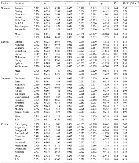
Table 4
Coefficients and statistics for estimation of solar radiation by Eq. (8), using both temperature and rainfall data
Region Location a b c d e f g R2 RMSE (MJ m−2)
Northern Broome 0.785 0.842 0.559 −0.055 −0.110 −0.143 −1.619 0.63 2.35 Cowley 0.576 0.026 2.339 0.017 −0.006 −0.137 −0.441 0.76 2.70 Cloncurry 0.570 0.003 2.468 0.003 −0.023 −0.194 4.861 0.66 2.87 Darwin 0.919 0.179 1.200 −0.008 −0.080 −0.128 −4.748 0.49 2.35 Halls Creek 0.644 0.006 2.312 0.008 −0.073 −0.125 3.419 0.74 2.09 Innisfail 0.685 0.038 1.667 0.043 0.001 −0.080 0.195 0.82 2.36 Rockhampton 0.700 0.026 1.874 0.034 −0.038 −0.124 −0.020 0.77 2.58 Townsville 0.916 0.122 1.429 −0.007 −0.072 −0.100 −6.477 0.63 2.98 Mean 0.724 0.155 1.731 0.004 −0.050 −0.129 −0.604 0.69 2.53
S.D. 0.138 0.284 0.657 0.030 0.040 0.033 3.775 0.11 0.30
Eastern Brisbane 0.714 0.023 2.076 0.030 −0.040 −0.109 −1.172 0.78 2.84 Nambour 0.732 0.143 0.975 0.011 −0.030 −0.139 0.482 0.70 2.86 Canberra 0.797 0.107 1.038 0.053 −0.015 −0.167 −0.480 0.86 2.90 Condobolin 0.812 0.728 0.388 −0.086 −0.224 −0.007 −1.654 0.82 3.15 Horbart 0.649 0.117 1.257 0.010 0.004 −0.164 −0.356 0.81 3.01 Melbourne 0.685 0.251 0.939 0.021 −0.040 −0.228 −0.933 0.77 3.39 Orange 0.503 0.328 0.968 −0.059 −0.185 −0.030 2.213 0.72 2.80 Sydney 0.737 0.109 1.569 0.006 −0.059 −0.155 −2.028 0.78 3.35 Williamtown 0.726 0.069 1.475 0.013 −0.022 −0.158 −0.700 0.77 3.30 Mean 0.706 0.208 1.187 0.000 −0.068 −0.129 −0.514 0.78 3.07
S.D. 0.091 0.216 0.479 0.044 0.080 0.070 1.259 0.05 0.24
Southern Geraldton 0.746 0.090 1.428 0.033 −0.033 −0.139 −0.501 0.85 2.76 Perth 0.715 0.061 1.438 0.013 −0.051 −0.158 −0.125 0.88 2.69 Wundowie 0.660 0.100 1.078 −0.016 −0.012 −0.177 1.620 0.89 2.40 Adelaide 0.783 0.236 0.964 0.025 −0.152 −0.001 −1.789 0.81 3.49 Albany 0.740 0.103 1.141 0.002 −0.098 0.000 0.079 0.82 2.90 Esperance 0.752 0.179 1.162 0.005 −0.016 −0.117 −2.262 0.82 3.08 Glen Osmond 0.666 0.060 1.683 −0.002 −0.011 −0.251 0.997 0.82 3.44 Hamilton 0.799 0.153 0.860 0.023 0.012 −0.158 0.436 0.82 3.38 Kyabram 0.827 0.426 0.516 −0.048 −0.183 0.015 −0.979 0.85 3.07 Laverton 0.714 0.124 1.132 0.007 −0.014 −0.193 −0.382 0.79 3.35 Mildura 0.742 0.032 1.618 0.010 0.026 −0.178 −0.365 0.87 2.80 Wagga Wagga 0.745 0.026 1.673 0.019 −0.014 −0.193 0.214 0.88 2.98 Mean 0.741 0.133 1.224 0.006 −0.046 −0.129 −0.255 0.84 3.03
S.D. 0.049 0.111 0.356 0.022 0.065 0.087 1.083 0.03 0.34
Central Alice Spring 0.756 0.016 1.840 0.029 −0.037 −0.188 0.462 0.85 2.47 Kalgoorlie 0.715 0.017 1.959 0.011 −0.044 −0.198 0.256 0.88 2.60 Longgreach 0.775 0.013 1.931 0.017 −0.027 −0.144 −0.844 0.86 2.23 Part Hedland 0.779 0.090 1.442 0.022 −0.072 −0.129 −1.976 0.78 2.47 Carnarvon 0.881 0.162 1.468 0.012 −0.040 −0.112 −5.306 0.86 2.54 Forrest 0.707 0.033 1.592 0.029 −0.020 −0.162 0.287 0.84 2.89 Learmonth 0.809 0.105 1.296 0.035 −0.077 −0.123 −1.748 0.86 2.43 Meekatharra 0.729 0.010 2.172 0.023 −0.025 −0.186 1.086 0.88 2.43 Oodnadatta 0.740 0.014 2.016 0.019 −0.035 −0.205 0.051 0.86 2.72 Woomera 0.707 0.016 2.083 0.011 −0.022 −0.192 0.442 0.86 2.80 Mean 0.760 0.048 1.780 0.021 −0.040 −0.164 −0.729 0.85 2.56
the radiation decreased by an average of 5%, while if rainfall was recorded at 09.00 h on the next day, the radiation was reduced by an average of 14%. The rain-fall recorded at 09.00 h on the next day most likely fell on the day of interest as we have not displaced the conventional records by 1 day (see Section 2.1). This suggested that rainfall recorded on the morning of the following day had a greater effect on the ra-diation than on the mornings of the current day and the day before. Another analysis was conducted to test if the rainfall recorded on the second and third day after had an effect on solar radiation on the cur-rent day. The analysis showed that there was no re-lationship between the radiation on the current day and the rainfall recorded on the second or third day following. Among the 3 days, contribution of dRj−1
was smallest, with a range between−0.09 and 0.05. In some sites at extremes of d values, the contribu-tion of dRj−1 was significant (P ≤ 0.001) in
im-proving the model performance; for example, at Con-dobolin if the rainfall was recorded on the previous day, Q was reduced by 9%. Further analysis showed that Eq. (8) with the term dRj−1 significantly (P ≤
0.01) improved the fit at 13 out of 39 sites. We, there-fore, reported 3-day rainfall for consistency across the sites.
As with the comparison in climatic regions, mean
R2in the northern region were 0.6, 0.48 and 0.69 for Eqs. (1), (5) and (8), respectively (Tables 2–4). The mean R2 increased to 0.82, 0.77 and 0.85 in central and similar values in southern region. Thus, >75% of total variance in measured radiations was accounted for by these models in central and southern regions and <70% was accounted in the northern zone. In general, RMSE in the northern and central zones were lower than eastern and southern zones. Compared with the overall mean values over the three models, R2 was 0.59, 0.72, 0.80 and 0.81 and RMSE was 2.77, 3.30, 3.21 and 2.74 MJ m−2for northern, eastern, southern and central regions, respectively. Estimates of Q across Australia had an overall mean R2of 0.75 and RMSE of 2.97 MJ m2 by Eq. (1), R2 of 0.68 and RMSE of 3.25 MJ m−2 by Eq. (5) and an averaged R2 of 0.80 and RMSE of 2.79 MJ m−2by Eq. (8). Thus, the three equations selected for dealing with various situations can provide considerably accurate estimations of solar radiation across Australia, where some daily radiation record was available.
The R2 and RMSE by Eq. (8) were 18 and 16% better, respectively, than that obtained using Eq. (5), while the improvement was 7% better than that using temperature only (Eq. (1)). This ranged from 15% in northern to 4% in the southern and central regions. The F-test for comparison of estimates between equa-tions showed that at 28 sites Eq. (8) significantly (P ≤ 0.01) improved the estimations over Eq. (1), while at six sites Eq. (1) was significantly better than Eq. (8). The six sites were all coastal and including Townsville, Sydney, Adelaide, Esperance, Carnarvon and Port Hedland. However, Eq. (8), compared to Eq. (1), has four additional parameters and requires rainfall data. Using the same standard comparison, Eq. (8) was 9 and 11% improvement over Eqs. (6) and (7), respectively. Eq. (6) was considered by Hay-hoe (1998) to be superior to WXGEN (Sharpley and Williams, 1990a,b), while Eq. (7) was the best model among five models evaluated by Hunt et al. (1998). Thus, Eq. (8) has remarkable improvement over the existing empirical models. This was largely attributable to the model incorporating the range of daily air temperature extremes (Bristow and Camp-bell, 1984) with rain-day data (McCaskill, 1990a,b).
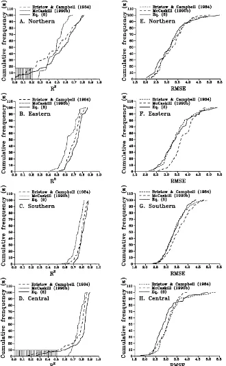
In the case of unavailable radiation data for devel-oping coefficients for a site, Fig. 5 showed the results obtained by applying the coefficients generated at one site to other sites within the same climatic region. The outcomes showed a higher degree of reliability in generating radiation without using the site calibration data in the eastern region (Fig. 5B and F) and south-ern region (Fig. 5C and G) than in the northsouth-ern region (Fig. 5A and E) and central region (Fig. 5D and H). Within northern region (Fig. 5A), more than 70% of
R2values were higher than 0.4 when radiation was es-timated by applying the coefficients from other sites. Within the central zone, over 90% of R2 were >0.4 (Fig. 5D). Within eastern region (Fig. 5B) the values of all R2 were >0.4 and within the southern region (Fig. 5C) they were all >0.6. In general, using rainfall only (Eq. (5)) the estimates of Q resulted in lower R2 in most of cases than the models either using temper-ature (Eq. (1)) or using both tempertemper-ature and rainfall (Eq. (8)). This may be because D accounted for vari-ation in radivari-ation due to cloud cover in sky was better than rainfall which can fall at night.
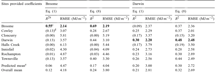
Table 5
Statistics for estimates of solar radiation for Broome and Darwin by regression coefficients obtained in the tropicsa
Sites provided coefficients Broome Darwin
Eq. (1) Eq. (8) Eq. (1) Eq. (8)
R2b RMSE (MJ m−2) R2 RMSE (MJ m−2) R2 RMSE (MJ m−2) R2 RMSE (MJ m−2)
Broome 0.55c 2.14 0.69 2.19 (0.09) 2.37 0.37 2.36
Cowley (0.13)d 3.07 0.28 2.67 0.25 2.29 0.37 2.01
Cloncurry (0.00) 5.81 (0.00) 5.19 (0.17) 3.37 (0.15) 3.20
Darwin (0.13) 3.57 0.44 3.10 0.30 2.20 0.48 2.48
Halls Creek (0.00) 6.13 (0.00) 5.44 (0.17) 3.79 (0.19) 3.50
Innisfail (0.02) 4.30 (0.04) 4.09 0.24 2.73 0.28 2.58
Rochampton (0.01) 4.87 (0.03) 4.46 0.23 3.16 0.30 2.89
Townsville (0.13) 3.57 0.40 3.30 0.26 2.56 0.44 2.49
Predicted meane 0.06 4.47 0.17 4.04 0.20 3.00 0.30 2.72
Overall mean 0.12 4.18 0.24 3.80 0.21 2.81 0.32 2.69
aThe two sites were the poorest predictions by coefficients from other sites in the northern regime. bThe R2 was the correlation coefficients between estimatedQand independent measuredQ. cThe values in bold are results by using the regression coefficients of its own site.
dThe values in the brackets areR2<0.2 which fill in the shaded area of Fig. 5a. eExclusive of the value obtained at its own site.
both temperature and rainfall (Eq. (8)) were evidenced for a few sites. These sites were for Broome and Dar-win in the northern region, the R2of which was shown in the shaded area of the CF in the Fig. 5A. There was poor performance for estimates of Q at Broome by regression coefficients obtained at other sites in north-ern region using Eq. (1) since all values of R2 were <0.2 with a mean of 0.06 (Table 5). However, there was a better performance by Eq. (8) using the coeffi-cients of Cowley (R2 =0.28), Darwin (R2 =0.44) and Townsville (R2=0.40). The estimates of Q for Darwin by Eqs. (1) and (8) were also relative poor. The R2of<0.2 for estimates of Q at this site resulted from using the coefficients from Broome, Cloncurry and Halls Creeks by Eq. (1) and the latter two sites by Eq. (8) (Table 5). Estimates of Q at the two sites using the coefficients obtained at the same sites were adequate, although only R2value of 0.3 was obtained for Darwin by Eq. (1). The associated RMSE for es-timates of Q for Broome by using Eq. (1) were rel-atively higher than other sites (Table 5). The poorest estimates for these two sites were by using the coef-ficients from the inland sites of Cloncurry and Halls Creek. The R2between the estimated Q and recorded
Q were 0.00 for Broome and<0.2 for Darwin. Thus, estimates of Q at Broome and Darwin should only use
the coefficients from their own sites, and certainly not from inland sites.
Table 6
Statistics for estimating solar radiation for Carnarvon by regression coefficients obtained in central regimea
Sites provided coefficients Eq. (1) Eq. (8)
R2b RMSE (MJ m−2) R2 RMSE (MJ m−2)
Alice Spring (0.20)c 5.00 (0.26) 4.72
Longreach (0.15) 5.30 (0.24) 5.00
Port Hedland 0.68 2.77 0.78 2.61
Carnarvon 0.79d 2.66 0.86 2.62
Forrest (0.28) 4.22 (0.40) 3.83
Kalgoolie (0.20) 5.16 (0.32) 4.66
Learmonth 0.61 3.28 0.75 2.82
Meekatherra (0.21) 5.40 (0.21) 5.30
Oodnadatta (0.18) 5.37 (0.27) 4.94
Woomera (0.28) 4.73 (0.40) 4.28
Predicted meane 0.31 4.58 0.40 4.24
Overall mean 0.36 4.44 0.45 3.08
aCarnarvon was the poorest predicted site by the coefficients from other sites in the central regime. bThe R2was the correlation coefficients between estimated Q and independent measured Q. cThe values in the bracket areR2<0.6 which fill in the shade area of Fig. 5d.
dThe values in bold are results by using the regression coefficients of its own site. eExclusive of the value obtained at its own site.
sites (Fig. 6A–C) and inland sites by the parameters of inland sites (Fig. 6D–F) against the distance between sites. The values of R2 (Fig. 6) or RMSE (Fig. 7) showed no relationship with the distance between the sites providing model parameters and sites for which the parameters were used to estimate solar radiation. This is different from the results reported in Canada by Hunt et al. (1998) which showed a linear increase in RMSE and linear decline in R2 with increase in distance between sites.
At coastal sites, R2 of 0.63 for estimates of Q by rainfall model (Eq. (5)) was smaller than the val-ues of 0.65 and 0.7 for estimates of Q by tempera-ture model (Eq. (1)) and both temperatempera-ture and rain-fall model (Eq. (8)), respectively. However, the rainrain-fall model was more reliable than the temperature model (Eq. (1)) and temperature-rain model (Eq. (8)), as R2
ranged between 0.27 and 0.83 using rainfall model, compared to the R2ranges from 0.02 to 0.89 by tem-perature and temtem-perature–rainfall models. In inland (Fig. 6D–F), R2for the three models ranged in a nar-rower and higher values than coastal sites with the best performance of temperature-rainfall model (Fig. 6F, R2=0.83), and the poorest using the rainfall model (Fig. 6E,R2=0.73). In the inland sites, Halls Creek and Cloncurry from northern and Orange from eastern region were the poorest predicted by all three
mod-els. These three sites have relatively high elevations in their respective regions (Table 1). However, the el-evations (altitude) did not effect the predicability of sites in all regions. This demonstrated that radiation for inland sites could be predicted with high accu-racy, with absence of measured radiation data. This can be useful as most crops are grown in the inland and simulations are often required to address various issues.
4. Conclusions
model (Eq. (1)) can be used with considerable accu-racy. When measurement of radiation data at the site was never done, coefficients used for estimation of Q within eastern or southern regions were more reliable than coefficients used for estimates of Q within north-ern and central regions. The estimations of Q can be improved if the coefficients of the models from inland sites are used for inland and those from coastal sites are used for coastal. For the coastal sites of the north-ern region, if estimates of Q have to be based on other sites, use the rainfall model, as it can provide more reliable estimates. At the inland of northern regions and central regions, Eq. (8) should be first considered, then temperature model or rainfall model, depending on the availability of data.
Acknowledgements
NSW Agriculture fully supported the research. The authors thank Dr. B.R. Cullis and Dr. K.H. Helyar, and G.M. Murray for statistical advice and comments.
References
Atwater, M.A., Ball, J.T., 1981. Effects of clouds on insolation models. Solar Energy 27, 37–44.
Australian Bureau of Meteorology, 1997. Climate Activities in Australia 1997: A report on Australian Participation in International Scientific Climate Programs. Bureau of Meteorology, Melbourne, 173 pp.
Boisvert, J.B., Hayhoe, H.N., Dube, P.A., 1990. Improving the estimation of global solar radiation across Canada. Agric. For. Meteorol. 52, 275–286.
Bristow, K., Campbell, G.S., 1984. On the relationship between incoming solar radiation and daily maximum and minimum temperature. Agric. For. Meteorol. 31, 159–166.
De Jong, R., Stewart, D.W., 1993. Estimating global solar radiation from common meteorological observations in western Canada. Can. J. Plant Sci. 73, 509–518.
Donnelly, J.R., Moore, A.D., Freer, M., 1997. DSS GRAZPLANT: Decision Support Systems for Australian Grazing Enterprises. I. Overview of the GRAZPLANT Project, and a Description of the MetACCESS and LambAlive. Agric. Syst. 54, 57–76. Duffie, J.A., Beckman, W.A., 1980. Solar Engineering of Thermal
Processes. Wiley, New York, 109 pp.
Fitzpatrick, E.A., Nix, H.A., 1970. The climatic factor in Australian grassland ecology. In: R. Milton Moore (Ed.), Australian Grasslands. Australian National University Press, Canberra, pp. 3–26.
Hargreaves, G.L., Hargreaves, G.H., Riley, J.P., 1985. Irrigation water requirement for Senegal River Basin. J. Irrig. Drain. Eng., ASCE 111, 265–275.
Hayhoe, H.N., 1998. Relationship between weather variables in observed and WXGEN generated data series. Agric. For. Meteorol. 90, 203–214.
Hook, J.E., McClendon, R.W., 1992. Estimation of solar radiation data missing from long-term meteorological records. Agron. J. 84, 739–742.
Hunt, L.A., Kuchar, L., Swanton, C.J., 1998. Estimation of solar radiation for use in crop modelling. Agric. For. Meteorol. 91, 293–300.
Huxley, P.A., 1973. Incoming solar radiation and degree-hours of temperature near Kampala Uganda. Agric. Meteorol. 11, 437– 443.
McCaskill, M.R., 1990a. An efficient method for generation of full climatological records from daily rainfall. Aust. J. Agric. Res. 41, 595–602.
McCaskill, M.R., 1990b. Prediction of solar radiation from rainday information using regionally stable coefficients. Agric. For. Meteorol. 51, 247–255.
Meinke, H., Carberry, P.S., McCaskill, M.R., Hills, M.A., McLeod, I., 1995. Evaluation of radiation and temperature data generators in the Australian tropic and sub-tropics using crop simulation models. Agric. For. Meteorol. 72, 293–316.
Nicks, A.D., Harp, J.F., 1980. Stochastic generation of temperature and solar radiation data. J. Hydrol. 48, 1–17.
Richardson, C.W., 1981. Stochastic simulation of daily precipitation, temperature, and solar radiation. Water Resources Res. 17, 182–190.
Richardson, C.W., 1985. Weather simulation for crop management models. Trans. ASAE 28, 1602–1606.
Richardson, C.W., Wright, D.A., 1984. WGEN: a model for generating daily weather variables. US Dept. Agric., Agric. Res. Ser., ARS-8, 83 pp.
Schulze, R.E., 1976. A physically based method of estimating solar radiation from suncards. Agric. Meteorol. 16, 85–101. Sharpley, A.N., Williams, J.R. (Eds.), 1990a. EPIC — Erosion/
Productivity Impact Calculator. 1. Model Documentation. US Dept. Agric. Techn. Bull. No. 1768, 235 pp.
Sharpley, A.N., Williams, J.R. (Eds.), 1990b. EPIC — Erosion/Productivity Impact Calculator. 2. User Manual. US Dept. Agric Techn. Bull. No. 1768, 127 pp.
Wallis, T.W.R., Griffiths, J.F., 1995. An assessment of the weather generator (WXGEN) used in the erosion/productivity impact calculator. Agric. For. Meteorol. 73, 115–133.