DIGITAL TERRAIN FROM A TWO-STEP SEGMENTATION AND OUTLIER-BASED
ALGORITHM
Mr. Kassel Hingeea,b,c, Dr. Peter Caccettab, Prof. Louis Caccettac, Dr. Xiaoliang Wub, Dr. Drew Devereauxb
a
School of Mathematics and Statistics, University of Western Australia, Stirling Highway, Perth, Western Australia [email protected]
b
CSIRO, Underwood Ave, Floreat, Perth, Australia -{Peter.Caccetta, Xioaliang.Wu, Drew.Devereaux}@csiro.au c
Department of Mathematics and Statistics, Curtin University, Kent Street, Bentley, Western Australia [email protected]
Commission III, WG III/2
KEY WORDS:Digital Elevation Models, DEM, DTM, DSM, ground filter, surface fitting, point cloud filtering
ABSTRACT:
We present a novel ground filter for remotely sensed height data. Our filter has two phases: the first phase segments the DSM with a slope threshold and uses gradient direction to identify candidate ground segments; the second phase fits surfaces to the candidate ground points and removes outliers. Digital terrain is obtained by a surface fit to the final set of ground points. We tested the new algorithm on digital surface models (DSMs) for a9600km2region around Perth, Australia. This region contains a large mix of land uses (urban, grassland, native forest and plantation forest) and includes both a sandy coastal plain and a hillier region (elevations up to 0.5km). The DSMs are captured annually at0.2mresolution using aerial stereo photography, resulting in1.2TB of input data per annum. Overall accuracy of the filter was estimated to be89.6%and on a small semi-rural subset our algorithm was found to have40% fewer errors compared to Inpho’s Match-T algorithm.
1. INTRODUCTION
Digital Elevation Models (DEMs) are important for studies of earth surface processes such as geomorphology, hydrology (Wil-son and Gallant, 2000) and vegetation (Moore et al., 1991). They also have applications in wireless communication (Sawada et al., 2006) and land cover map generation (Caccetta et al., 2015). It is popular to generate DEMs using remote sensors including light detection and ranging sensors (LiDAR), digital stereo (multiple view)-photography, and interferometric synthetic aperture radar (InSAR). Such sensors may be airborne or spaceborne and pro-vide dense observations of the land surface. From the data ac-quired, positional (e.g. x,y,z) and surface property (e.g. reflectance from optical photogrammetry or backscatter from SAR) informa-tion is directly available, or with some processing, may be de-rived. The positional information is directly relevant to the gen-eration of a Digital Surface Model (DSM), which records heights of any feature relative to a reference (typically taken to be zero at mean sea level). In this paper we focus on the generation of Dig-ital Terrain Models (DTM), which provide estimates of ground elevation, through filtering and then removing above ground ob-jects from DSMs. We note that given a DSM and a DTM, then we may derive a so called “normalised Digital Surface Model” (nDSM) by simple subtraction of the DTM from the DSM. DTMs are typically used for estimating ground properties such as deriva-tives (slopes and curvatures) or flow path prediction in runoff models. nDSMs are typically used for building and/or tree height extraction.
The published literature is mostly focused on LiDAR data, how-ever many of the concepts and results generalise to stereo pho-tography derived point clouds due to the similarities of the sensed objects. Meng et al. review and comment on the existing meth-ods for ground filtering LiDAR point clouds (Meng et al., 2010). They categorised algorithms into six classes, segmentation/clus-tering, morphological, directional scanning, contour-based, TIN-based and interpolation-TIN-based. We prefer a coarser classification:
algorithms either label individual points, or label clusters or seg-ments of points. Furthermore this labelling is performed using neighbourhood based comparisons (e.g. morphological and direc-tion scanning) and/or surface-based comparisons (contour, TIN and interpolation based). Alternative classifications are given by (Shan and Aparajithan, 2005) and (T´ov´ari and Pfeifer, 2005).
Neighbourhood comparisons typically use operators derived from the morphological opening and closing operations to quickly la-bel points as ground. In comparison, algorithms that lala-bel seg-ments/clusters such as (Belkhouche et al., 2015) and (T´ov´ari and Pfeifer, 2005), divide the point cloud into homogeneous groups of points and then use neighbourhoods, fitted surfaces or proper-ties of the segments to discriminate ground segments from non-ground segments.
The review article (Sithole and Vosselman, 2004) lists common difficulties for ground filters of LiDAR data:
• Outlying pointsfar above or below the true surface. These are usually caused by sensor or matching errors, or birds or aircraft in the image. Most filters have a bias towards low points so low outliers are typically more problematic than high outliers.
• Large objects.These are especially problematic for filters that use fixed-sized neighbourhoods because the object’s extents may exceed the neighbourhood.
• Complex shapes and configurations. For example, discon-nected patches of bare earth (such as courtyards), build-ings connected to other buildbuild-ings, roofs that have multiple levels, or roofs overshadowed by trees.
• Attached objectsare objects that are seamlessly connected to the ground on one edge, but are above the ground on another edge. Some examples of this are roofs that touch the ground, bridges and ramps.
• Vegetation on slopes or low vegetation. It is difficult to determine between natural variation in the Earth’s surface and variation due to vegetation.
• Discontinuities and abrupt height changesin the ground. Many filters remove or smooth these terrain features.
For stereo photography data, canopies also present difficulties be-cause stereo photography relies on observations from two or more views potentially producing fewer ground points than LiDAR.
There are two types of errors in classifying ground points: omis-sion errors (rejection of true bare-Earth points) and commisomis-sion errors (false labelling of objects as bare-Earth).
This paper presents a novel algorithm for generating DTMs from DSMs. We concentrate our description on using elevation models presented in raster/gridded form, and note that the concepts gen-eralise to non-gridded points. The algorithm first labels segments and then applies a surface-based outlier removal. It differs from the algorithm of (Woestyne et al., 2004) by using (1) a neigh-bourhood to label the segments so that small isolated patches of ground are correctly filtered and (2) a multiresolution out-lier removal that can quickly remove large regions of non-ground points. The algorithm is described in detail in Section 2.
We applied the algorithm to a 9600km2 decimetre resolution dataset and the quality of the resulting DTMs are discussed in Section 3. The filter accuracy was89.6%and the DTMs are al-ready in use by local governments (Western Australian Planning Commission, 2013).
2. MATERIALS AND METHODS
Here we describe our 2-stage algorithm for generating DTMs from DSMs. The complete work flow is presented in Figure 1. The data used for developing and testing the algorithm is described in Section 2.1. The surface fitting algorithm used in both the surface-based filter and the final DTM interpolation is described in Section 2.2. The first stage comprises a segment-labelling neighbourhood filter and is described in Section 2.3. The second stage, a point-labelling surface-based filter, is de-scribed in Section 2.4. Computational aspects of producing the DTMs are described in Section 2.5.
Stereo
surface fitting and outlier removal 1a) multiresolution surface fit
. REPEAT 6 TIMES IN TOTAL .
Figure 1. Complete work flow from stereo photography to DTM
2.1 Data
The algorithm can be applied directly to point clouds generated by LiDAR or stereo photography, however for simplicity we use DSMs that are already available.
The DSMs were generated as part of a wide-region, fine-scale ur-ban monitoring study (Caccetta et al., 2015). See Figure 2 for an example DSM. This project leverages state-funded annual stereo aerial photography capture of a9600km2 region around Perth, Australia. Henceforth we will refer to this region as the Urban Monitor (UM) region.
The annual stereo aerial photography data set, which contained approximately 35,000 frames per annum, was acquired using a Microsoft UltraCAM-D (Leberl and Gruber, 2003) flown at a height of about 1300m above the ground, capturing multispec-tral data (red, green, blue and near infrared bands) along with panchromatic data. The ground sample distance (GSD) was ap-proximately0.3mand0.1mfor the multispectral and panchro-matic data respectively. The dates of each capture corresponded to Perth’s dry hot Mediterranean-type summers. The captured frames had at least 65% forward and 30% side overlaps. The overlaps among frames allowed detailed DSM to be extracted us-ing stereo photogrammetric techniques.
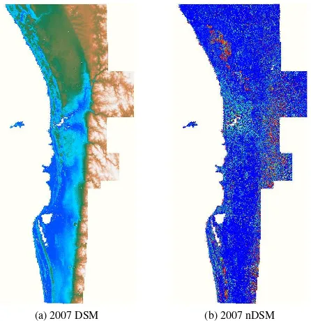
(a) 2007 DSM (b) 2007 nDSM
Figure 2. The UM region. It is 210kmfrom North to South. Viewed at this scale the DSM (a) is indistinguishable from the DTM, instead we show the nDSM (b). In the nDSM cool colours correspond to low elevations, hot colours are high elevations (red = taller than10m). Noticeable are tall canopies of dense plan-tation forests in the North, and non-uniform canopy of native forests in the East. Some height errors in water are also visi-ble due to DSM issues over water. In (a) elevations range from 0m(blue) to approximately0.5km(white) above sea level.
2.2 Multi-Resolution Surface Fitting
The surface fitting algorithm was derived from Terzopoulos’ work (Terzopoulos, 1988) and is quite similar to the surface fitting al-gorithms of Bolitho et al. (Bolitho et al., 2007) and Zoraster (Zo-raster, 2003). The algorithm can be applied directly to a point cloud to generate a DSM. In principle other surface fitting meth-ods might also be sufficiently fast and accurate.
The algorithm operated at multiple resolutions using coarse res-olution results as starting estimates for fine resres-olution surface fit-ting. The surface fitting at a coarse resolution provides approxi-mate surfaces with relatively small computational costs. The finer resolution surface fitting adjusts this approximate surface to im-prove detail and accuracy. Multiple resolution algorithms are well known for reducing computation times.
At each resolution the initial surface guess was iteratively evolved to minimise an energy function that combined a data matching cost with a roughness cost. The former was the difference be-tween the estimated surface and the input points averaged to the current resolution. The latter was based on the magnitude of the second-order derivatives of the surface.
Further details may be found in (Hingee, 2013) and a forthcoming paper (Hingee et al., 2016).
2.3 Segmentation Filter
This filter used an algorithm known as inflowsthat was origi-nally developed by one of the authors (Caccetta, 1997). Sim-ilar algorithms were more recently presented for point clouds (Belkhouche et al., 2015) and DSMs (Beumier and Idrissa, 2015). The filter required a slopeSparameter, an areaAparameter and
a relative gradientRparameter to be provided by the user. The algorithm first labelled pixels having slope less thanSas candi-date ground points (cgp), and rejected all other pixels. Connected components of cgp were treated as regions. Regions with area smaller thanAwere rejected, largely for the purpose of remov-ing numerous commission errors at the expense of some omis-sion errors. Remaining regions were then labelled according to the percentage of neighbouring boundary pixels higher than the nearest region pixel, or in watershed terminology, the percent-age of neighbouring pixels that would flow into the region (hence the term “inflow”). Regions having inflow scores greater than, for exampleR = 0.5, were retained and all other regions were rejected. An example is shown in Figure 3.
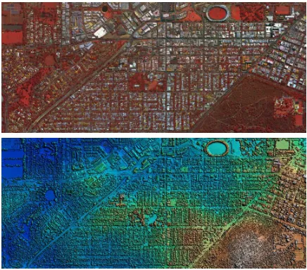
(a) true colour (b) sun shaded DSM
(c) inside inflows (d) ground mask (in pink)
Figure 3. An example of the inflows segmentation filter in action. Using the DSM (b) (hot/grey colours correspond to high DSM values), the area was segmented into pixels above or below the slope threshold (c). In (c) pixels that would ‘flow’ into a neigh-bouring region are yellow, and pixels that would ‘flow’ away from a neighbouring region areblue. In (c) the level segments are coloured with various saturations of red; the less saturated (darker) a segment the higher the proportion of inward flowing pixels. The segments with more than 50% of their boundary pix-els flowinginwardswere then labelled ground (d) (ground pixels are coloured pink).
The parameters used for the UM region wereS = 25o
, A = 0.4m2andR= 0.5. Initial testing indicated that the algorithm performed well on outliers in the DSM, discontinuities, sharp ridges, low vegetation, vegetation on slopes, large objects, and even low objects. However it often misclassified saw-toothed roofs, attached objects (such as roof-top car parks) and more complex configurations such as roofs with many objects on top of the roof and roofs neighboured by even higher roofs (such as in high density commercial districts). It also had difficulty with large horizontal segments in canopies (where the areas of segments could be greater than the area threshold ofA) and ex-tremely steep terrain (greater thanSslopes).
With inflows as the only filter these few (by area) commission errors resulted in DTMs with mounds every few metres, see Fig-ure 4 for an example. Initial testing suggested that this was an unacceptable error rate, however inflows was extremely fast.
Removal of further non-ground points required a method that compared candidate points to the closest true-ground points, which were potentially many metres to tens of metres away. This suggested either extremely large neighbourhoods (larger than most non-ground objects) or surface fitting. In the next section we describe our solution which was based on the latter.
2.4 Surface-based filter
(a) False Colour (b) DSM (c) Candidate Ground Points
(d) Fitted Surface
Figure 4. An example of a surface fitted to an inflows candidate ground mask. Shown is a false colour display of the region (a), the DSM (b), the set of cgp from inflows (c) and the fitted surface (d). The sub-figures (b), (c) and (d) are coloured according to the same height scale (blue = low, red = high). The surfaces (a) and (d) are also sun-shaded to accentuate texture. In (c) the black pixels are those that were not candidate ground. A few high, non-ground, pixels (coloured green or yellow due to their height) can be seen in (c); they are causing the large mound-like features in (d).
second-order derivatives,
∂2u
∂x2 2
+ 2
∂2u
∂x∂y
2 +
∂2u
∂y2 2
,
evaluated at(i, j)(calculated by discrete approximation from the heights of neighbouring pixels) was above a user-defined thresh-oldandthe cgp was above the fitted surface.
The protection of below-surface cgp prevented true-ground points from being removed when nearby above-ground points caused rough surfaces. In the present algorithm this caveat was relaxed on some iterations to remove below-ground DSM errors which occasionally resulted in loss of true ground points.
2.4.1 Parameter Selection. The user defined thresholds were chosen by trial-and-error on small subsets of the data. The region contained two broad terrain types, a smooth coastal plain that contained most of the urban area and a hillier area with little ur-ban development and lots of forests. In Figure 2a the hillier area is mostly orange and white, whilst the plains are green and blue. Exploratory testing gave a strong indication that it would be ben-eficial to use different parameters for each of these terrain types. On the coastal plain there were many complicated aboveground structures (due to the higher urbanisation) leading to more com-mission errors by inflows, however the greater smoothness of the ground allowed stricter thresholds and thus enabled removal of more non-ground points.
Parameter choices in the surface fitting algorithm affected both the computation time and the quality of the filtering. A smoother surface used coarser resolutions, required less computation time, and enabled tighter roughness thresholds which removed larger amounts of commission error. However smoother surfaces were unable to detect small commission errors that were close to true-ground points. Heuristically, surface fitting at3.2mresolution (which was24 times the input DSM resolution) is ideal for re-moval of residential roof sized patches of commission error be-cause at this resolution a residential roof is only a few pixels wide and there are similar sized patches of ground (backyards, roads) to constrain the surface close to true ground. Outlier removal that used1.6mresolution or finer surface fits were useful because the surface fitting could detect a greater number of small commis-sion errors in trees. Outlier detection at the full0.2mresolution was not considered due to the greater computational time it re-quired. Furthermore additional care was taken when candidate
ground points below the surface could be removed because there was a risk that true ground points on the floors of valleys and depressions would also be removed.
We used two areas to guide parameter selection, a sharp, well vegetated valley for the hills (Figure 5) and a large region con-taining urban, suburban and parkland areas for the coastal plain (Figure 6). These regions were chosen to be challenging with the expectation that the filter will work better on any other region.
Only six iterations were used due to the complexity of determin-ing parameters. The parameters selected, and details of the pa-rameter search can be found in (Hingee, 2013). We do not in-clude them here because they were specific to the surface fitting program and do not add much conceptually.
(a) false colour display (b) sun-shaded DSM
Figure 5. The region used to guide parameter choices for the hilly terrain. Dimensions:1kmby1km. Grey colours correspond to high elevations (∼270m), cool colours correspond to low eleva-tions (blue∼63m).
Figure 6. The region used to guide parameter choices for the coastal plain. Shown is a false colour display (above) and sun-shaded DSM (below). Dimensions: 3.4kmby 1.4km. Grey colours correspond to high elevations (∼63m), cool colours cor-respond to low elevations (blue∼10m).
2.5 Processing
The surface-based outlier removal together with the final surface fit to produce a DTM required around 16GB of memory and just over 4 hours of CPU time for each tile resulting in over 4000 hours of processing in aggregate. In comparison the segment-labelling filter used very little memory or other resources.
The resulting DTM tiles were mosaicked back together to form the final DTM taking around 36 hours to complete. The 1000-pixel tile overlap allowed the feathering of edges through a simple linear weight ramp, from a weight of 0 at the edge of a tile, to 1 where the overlap finished. Without this feathering the final mosaic would have contained extensive tile edge effects, due to surface fitting being calculated independently on each tile.
The nDSM in Figure 2, which was generated by simply subtract-ing the DTM from the DSM, required around 5 hours to complete.
3. RESULTS AND DISCUSSION
The quality of the final DTMs generated for the region were in-vestigated with a manual inspection of the entire region (Section 3.1), arrays of manually classified points (Section 3.2) and a com-parison to the commercially available match-T algorithm (Sec-tion 3.3).
3.1 Manual Inspection
The DTMs of the entire UM area were manually inspected for large errors and large patches of errors. Here we focus on the DTM for 2007. The results of the other year, 2009, were similar - see (Hingee, 2013). Due to time constraints the DTM was only checked at scales larger than the typical residential house.
Industrial roofs were often problematic because inflows was con-fused by their complex shapes (saw-toothed roofs, rooftop car parks attached to the ground, and roofs with objects on them are all common in industrial/commercial zones) and the large roof areas hindered removal by the smoothing filter. Bridges were not classed as commission errors because in some real-life situations they are regarded as ground, however it was noticed that our filter partially commissioned most bridges as ground - inflows labelled them as ground and the smoothing filter eroded the edges.
Some dense forest issues also occurred, primarily in two large plantation forests, and were due to a lack of visible ground to constrain the surface-based filter.
Discontinuities and sharp changes in true ground such as cliffs, gullies and occasional peaks of sand dunes were overly smoothed however these issues were either small or rare, and deemed a rea-sonable price for reduced commission error.
Two large gentle hill-sides were interpolated instead of fitting to ground points present in the DSM. These were caused by large ground segments with inflow scores lower than the threshold of R= 0.5.
The effects of the piecewise generation of the DTM (recall that the size of the data necessitated surface fitting on4kmby4km subsets) were only noticed three times, all in large data-less re-gions such as rivers or lakes.
3.2 Comparison to Arrays of Manually Interpreted Points
In clear, flat, open ground, manual inspection showed that the DTM was nearly identical to the DSM and consequently inaccu-racies of the DTM were attributed to two sources, the input DSM
and any commission/omission errors of the ground filter (a third source, occlusions, was also possible in other parts of the UM region where there was very dense forest).
Accuracy was estimated by arrays of points in three separate re-gions. A complex urban region (the same region used to train parameters for the coastal plains), a simpler coastal suburb and a farming district that contained a nature reserve. Manual interpre-tation of these points as either ground, non-ground, or unknown (could not distinguish between ground or non-ground) was per-formed using orthorectified images. Due to time restrictions no manual interpretation of points occurred in the hilly region.
The difference of the final 2007 DTM to the 2007 DSM was thresholded at0.3mto label locations as ground/not-ground. This allowed investigation of the commission/omission of our ground filter, but not absolute accuracy of the DTM. See table 1 for the confusion matrix pooled across all three regions.
An overall accuracy of89.6%was achieved with a2.2% com-mission error and a8.1%omission error.
Differences in terrain complexity, sensor properties and prepro-cessing make comparison of these accuracies to published results difficult. Instead the next section presents a direct comparison to a commercially available DTM algorithm.
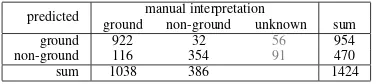
predicted manual interpretation
ground non-ground unknown sum
ground 922 32 56 954
non-ground 116 354 91 470
sum 1038 386 1424
Table 1. Confusion matrix for the 2007 DTM. The proportion of predictions that matched the manual interpretations (the over-all accuracy) was89.6%, the percentage of manually interpreted pixels that wereincorrectlypredicted asground(the commission error) was2.2%and the fraction of manually interpreted pixels that wereincorrectlypredicted asnon-ground(the omission er-ror) was8.1%(these accuracies and the sums of each row above are ignoring the unknown pixels).
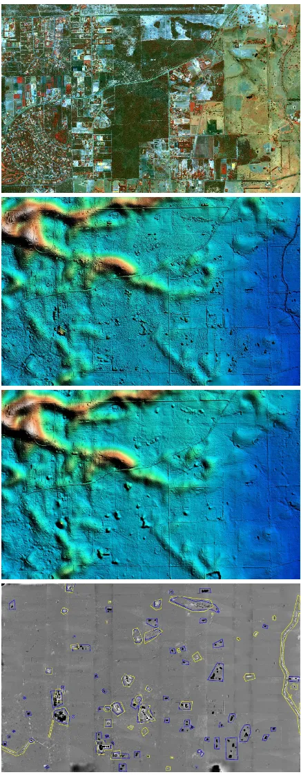
3.3 Comparison to an Inpho match-T DTM
Inpho’s match-T algorithm (Lothhammer, 2005) was used to cre-ate both a DSM and a DTM for a4.5kmby5.7kmregion repre-senting a fairly simple, but prevalent landscape. The region was on the flat coastal plain and contained clear ground, sparse forest and large, highly vegetated residential blocks. Due to time and data transfer limits it was only possible to compare algorithms on this small region.
Exactly the same raw photographs from the 2009 data were used for both algorithms. The default parameters were used for the Inpho algorithm. It is likely Inpho’s DTM could have been im-proved with better parameters however this risked over fitting.
In clear open ground both DTMs closely matched the DSMs so numerical height accuracies were not compared. However there were clear differences in the abilities of each method to filter non-ground objects.
The height of the two DTMs were then differenced (Figure 7, bot-tom) to highlight further differences, this was especially useful for discerning omission errors in our DTM. Differences that the user could not easily attribute as error, such as inclusion/exclusion of a large mound of dirt, were ignored.
Images of the results are shown in Figure 7. A total of40errors were found in our DTM. There were20commission errors of trees,15omissions of dams and gullies,3roofs commissioned as ground and2incidences where the DTM smoothed over true bulges in the ground.
A total of67errors were found in Inpho’s DTM. There were59 errors caused by trees,6roof errors, and2erroneous protrusions in the DSM that the DTM failed to remove. No omission errors were found; it did not smooth over gullies or dams.
Overall our algorithm resulted in40%fewer errors. Inpho’s DTM contained almost three times as many vegetation commission er-rors as our DTM, and twice as many roof erer-rors. However it captured many sharp changes in the ground, which were mostly caused by gullies and dam walls, that our DTM consistently mis-sed. In dense urban areas and forests Inpho is likely to create many more above-ground errors because there are many more above-ground objects in these regions. The improvement gained from our algorithm implies a significant reduction in costly man-ual editing for the region.
Assuming the accuracy of our DTM here is similar, on average, to the whole UM region the error counts suggest at least400 un-recorded small-scale commission errors.
4. CONCLUSION
Our algorithm’s estimated accuracy for the Perth region was 89.6% and in a peri-urban region it produced 40% fewer errors than Inpho’s match-T algorithm. Qualitative manual inspection suggested that the algorithm produced good estimates of ground height in well-vegetated dense suburbs, new suburbs, peri-urban areas and farmland. However it had difficulties with a few rarer terrains: industrial buildings, dense forests, extremely steep hills, sharp depressions and discontinuities.
The algorithm, which combines a segmentation filter with a sur-face based smoothness filter, shows how improvements to single method algorithms can easily be obtained through a secondary filter. It is also a rare demonstration of DTM estimation from digital stereo photography.
The results of this algorithm applied to the UM region are already in use by urban decision makers (Western Australian Planning Commission, 2013, page 13).
5. FUTURE WORK
In the future we would like to gain a better estimate of our algo-rithm’s accuracy using manually interpreted points over a broader region. We would also like to investigate improvements to the filter through a specialist below-ground filter and/or morphologi-cal removal of outliers after surface fitting. Applications to very steep terrains could use an inflows variation wherein segments of slowly changing slope are separated by high curvatures.
Our algorithm was sufficiently fast and accurate to produce DTMs for multiple dates. Future comparisons between these DTMs could provide further valuable information to a wide range of professionals.
ACKNOWLEDGEMENTS
Our thanks to Aaron Thorn and Landgate for generously provid-ing the Inpho DTM for Section 3.3. This work was also supported by resources provided by the Pawsey Supercomputing Centre with funding from the Australian Government and the Government of Western Australia.
REFERENCES
Abo Akel, N., Zilberstein, O. and Doytsher, Y., 2004. A robust method used with orthogonal polynomials and road network for automatic terrain surface extraction from LiDAR and urban ar-eas. In: International Archives of Photogrammetry and Remote Sensing, Vol. XXXV, Part B3, Istanbul, Turkey, pp. 243–248.
Belkhouche, Y., Duraisamy, P. and Buckles, B., 2015. Graph-connected components for filtering urban LiDAR data. Journal of Applied Remote Sensing9(1), pp. 096075–096075.
Beumier, C. and Idrissa, M., 2015. Deriving a DTM from a DSM by uniform regions and context. In:EARSeL eProceedings, Vol. 14, pp. 16–24.
Bolitho, M., Kazhdan, M., Burns, R. and Hoppe, H., 2007. Mul-tilevel streaming for out-of-core surface reconstruction. In: Pro-ceedings of the fifth Eurographics symposium on Geometry pro-cessing, Eurographics Association, pp. 69–78.
Caccetta, P., 1997. Remote sensing, geographic information sys-tems (GIS) and Bayesian knowledge-based methods for monitor-ing land condition. Phd, Curtin University of Technology. Thesis.
Caccetta, P., Collings, S., Devereux, A., Hingee, K., McFarlane, D., Traylen, A., Wu, X. and Zhou, Z., 2015. Monitoring land surface and cover in urban and peri-urban environments using digital aerial photography.International Journal of Digital Earth pp. 1–19.
Collings, S. and Caccetta, P., 2013. Radiometric calibration of very large digital aerial frame mosaics. International Journal of Image and Data Fusion4(3), pp. 214–229.
Collings, S., Caccetta, P., Campbell, N. and Wu, X., 2011. Em-pirical models for radiometric calibration of digital aerial frame mosaics.IEEE Transactions on Geoscience and Remote Sensing 49(7), pp. 2573–2588.
Hingee, K., 2013. Ground elevation models and land cover clas-sifiers for decimetre resolution urban monitoring. M. phil, Curtin University, Perth, Australia. (Thesis).
Hingee, K., Caccetta, P., Caccetta, L., Wu, X. and Deveraux, D., 2016. Digital terrain from a digital surface model: a two-step segmentation and outlier based algorithm. under review.
Kobler, A., Pfeifer, N., Ogrinc, P., Todorovski, L., Oˇstir, K. and Dˇzeroski, S., 2007. Repetitive interpolation: A robust algorithm for DTM generation from Aerial Laser Scanner Data in forested terrain. Remote Sensing of Environment108(1), pp. 9–23.
Lothhammer, K.-l., 2005. State-of-the-art photogrammetric workflow the inpho approach.Semana Geomaticapp. 1–9.
Moore, I. D., Grayson, R. B. and Ladson, A. R., 1991. Digital terrain modelling: A review of hydrological, geomorphological, and biological applications.Hydrological Processes5(1), pp. 3– 30.
Sawada, M., Cossette, D., Wellar, B. and Kurt, T., 2006. Analy-sis of the urban/rural broadband divide in canada: Using GIS in planning terrestrial wireless deployment. Government Informa-tion Quarterly23(3–4), pp. 454–479.
Shan, J. and Aparajithan, S., 2005. Urban DEM generation from raw lidar data.Photogrammetric Engineering & Remote Sensing 71(2), pp. 217–226.
Sithole, G. and Vosselman, G., 2004. Experimental comparison of filter algorithms for bare-Earth extraction from airborne laser scanning point clouds. ISPRS Journal of Photogrammetry and Remote Sensing59(1-2), pp. 85–101.
Terzopoulos, D., 1988. The computation of visible-surface rep-resentations. Pattern Analysis and Machine Intelligence, IEEE Transactions on10(4), pp. 417–438.
T´ov´ari, D. and Pfeifer, N., 2005. Segmentation based robust interpolation-a new approach to laser data filtering. In: Inter-national Archives of the Photogrammetry, Remote Sensing and Spatial Information Sciences, Vol. XXXVI-3/W19, pp. 79–84.
Vosselman, G., 2000. Slope based filtering of laser altimetry data. In:International Archives of Photogrammetry and Remote Sens-ing, Vol. XXXIII, Part B3, Amsterdam, p. 935–942.
Wang, C. and Tseng, Y., 2014. Dual-directional profile filter for digital terrain model generation from airborne laser scan-ning data. Journal of Applied Remote Sensing8(1), pp. 083619– 083619.
Western Australian Planning Commission, 2013. Capital City Planning Framework: a vision for Central Perth. Technical Re-port February, Western Australian Planning Commission, Perth.
Wilson, J. P. and Gallant, J. C. (eds), 2000. Terrain analysis: principles and applications. Wiley.
Woestyne, I. V. D., Jordan, M., Moons, T. and Cord, M., 2004. A software system for efficient DEM segmentation and DTM es-timation in complex urban areas. In:The International Archives of the Photogrammetry, Remote Sensing and Spatial Information Science, Vol. XXXV, Part B3, Istanbul, Turkey, pp. 134–139.
Wu, X., 1995. Grey-based relaxation for image matching. In: DICTA-95, Vol. 95, Brisbane, Australia.
Wu, X., 1996. Multi-point least squares matching with array re-laxation under variable weight models. In:International Archives of Photogrammetry and Remote Sensing, Vol. XXXI, Part B3, Vi-enna, p. 977–982.
Zoraster, S., 2003. A surface modeling algorithm designed for speed and ease of use with all petroleum industry data. Comput-ers & Geosciences29(9), pp. 1175–1182.