UPDATING LAND COVER DATABASES USING A SINGLE VERY HIGH RESOLUTION
SATELLITE IMAGE
Adrien Gressin1,2, Cl´ement Mallet1, Nicole Vincent2and Nicolas Paparoditis1
1IGN/SR, MATIS, Universit´e Paris-Est, 73 avenue de Paris, 94160 Saint-Mand´e, France;
2LIPADE - SIP, Paris-Descartes University, 45 Rue des Saint-P`eres, Paris, France; ([email protected])
KEY WORDS:change detection, updating, classification, image, 2D topographic database, very high resolution, satellite.
ABSTRACT:
Image change detection has been extensively tackled in the literature in various domains, and in particular for remote sensing purposes. Indeed, very high resolution geospatial images are nowadays ubiquitous and can be used to update existing 2D and 3D geographical databases. Such databases can be projected into the image space, by a rasterization step. Therefore, they provide 2D label maps that can be subsequently compared with classifications resulting for geospatial image processing. In this paper, we propose a classification-based method to detect changes between label maps created from 2D land-cover databases and an more recent orthoimage, without any prior assumptions about the databases composition. Our supervised method is based both on an efficient training set selection and a hierarchical decision process, that follows the structure of topographical databases. This allows to take into account the intrinsic heterogeneity of the objects and themes composing a database while limiting false detection rates, a standard limitation of existing approaches. The designed framework is successfully applied on very high resolution images of Pl´eiades sensor and two distinct national land-cover databases.
1 INTRODUCTION
2D topographic land-cover databases are now available over most of the extent of many developed countries. Such databases are mainly created by merging existing databases of various kinds and sources. Classes of high interest that are not in such databases are derived according to ground surveys, photo-interpretation of very high resolution images, or development of automatic theme-specific detection algorithms.
In France, the generation of the new global 2D land-cover/land-use (LC/LU) database at a spatial resolution of 1 m has started in 2013, on the initiative of several public institutions. It is or-ganised in a hierarchical manner, similarly to Corine Land Cover, so as to fit with a large number of users’ needs. Furthermore, it aims to federate various existing databases both at national and regional levels (buildings, roads, water areas, rivers, forests, agri-culture etc.). After the generation of the initial state, two issues remain challenging. First, the completeness and the geometrical accuracy of all the classes included in these databases may vary significantly and one has to detect discrepancies with respect to the database specifications. Secondly, such a database needs to be updated at least every year. Since most classes are the result of human intervention, automatic change detection processes should be set up and be valid for each of these labels.
The aim of this paper is to present a new method to solve both issues equally, using geospatial images at the same resolution as the LC/LU database, namely very high resolution satellite im-ages, without any prior assumption about the database classes. The recent launch of very high resolution (inferior to 1m) satellite sensors, such as Pl´eiades or Worldview-2, allow to obtain a reg-ular coverage of large areas in a very short period of time. How-ever, despite the ability of such sensors to acquire stereoscopic images, their scheduling and cost issues often limit the disposal to a single image per period (monoscopic configuration). In this paper, we will therefore focus on single images of sub-metric res-olution, regularly acquired over the year, to automatically update land-cover databases.
Change detection is a main subject of research in the image pro-cessing domain, e.g., for video surveillance, infrastructure
mon-itoring or medical diagnostic (Radke et al., 2005; Goyette et al., 2012). In remote sensing, a large body of literature has tackled the problem, from many points of view. For instance, changes can be detected between two images (Miller et al., 2005), or sev-eral high or very high resolution images (time-series) (Robin et al., 2010; Petitjean et al., 2012; Bovolo et al., 2013). Hussain et al. (2013) provide a good overview and taxonomy of change de-tection methods.
More specifically, detecting changes between a LC/LU database (DB) and images more recent than the images or the observa-tions that allowed to populate the DB is a main subject of interest (Holland et al., 2006; Gianinetto, 2008; Champion et al., 2010). For example, Marc¸al et al. (2005) match objects of a DB with image saliencies, in order to select good training sets for the su-pervised classification of a multi-spectral image, using Support Vector Machine and Logistic Discrimination methods. Walter (2004) segments aerial images according to DB object outlines and performs an object-based classification using a supervised Maximum Likelihood classification, eventually compared with the initial DB for change detection. More generally, one can no-tice that existing methods focus on a very specific object type (e.g., roads, buildings), and require the computation of 3D fea-tures from stereoscopic images, in order to better discriminate such objects (Nemmour and Chibani, 2006; Poulain et al., 2009; Champion et al., 2010). Helmholz et al. (2012) integrate such specific methods in a global semi-automatic workflow for detect-ing changes between a 2D geographical DB and orthorectified up-to-date images. Each object of the DB is verified by an auto-matic image analysis operator, integrated into a knowledge-based image interpretation system. This work is closely related to our issues, but specific methods have to be developed for each kind of label (also calledtheme) of the DB, and new classes would not be directly supported. Thus, this method cannot be adopted here. Finally, the analysis of the approaches mentioned above allows us to conclude that:
or unsupervised clustering approaches;
⊲As few changes exist between the DB and the image, the DB can be kept as initial solution to select reliable training sets for the classifier.
Such assumptions will be the basis of the solution proposed here. Nevertheless, contrary to approaches developed so far, our method targets to detect any change (new, modified, and deleted objects) from any theme of the DB of interest. The robustness of the change detection system will be mainly guaranteed by the selec-tion of the training sets that best discriminate each object of the DB from the rest of the image. Such a per-object consideration will then be propagated into the hierarchical layout of the DB by merging information at each DB level in order to strengthen the process. Our method introduces several new relevant features: ⊲No restricting inputs. A single very high resolution (<1m) satellite image is required, without stereoscopic configuration. To deal with such a weak input, a very high number of features are computed from the image, and we assume they will be sufficient to learn the visual aspect of the different themes of the DB; ⊲Independence to the objects of interest. Our feature set and training step are not designed for specific object types. Therefore, our method can be applied on any 2D geographical database; ⊲Theuse of the hierarchical layout of the DBallows a bottom-up analysis (object→theme→DB) and to obtain LC and change maps consistent with the different objects populating each theme of the DB.
An overview of our change detection methodology is first intro-duced in Section 2.1. Then, the hierarchical approach is detailed in Section 2.2. Results are presented for two different 2D topo-graphic databases at two different levels of details in Section 3. Finally, conclusions are drawn in Section 4.
2 METHODOLOGY
In this section, we first provide an overview of our methodology and introduce some notations. Then, the three levels of our ap-proach are detailed. Finally, technical choices are discussed.
2.1 Overview
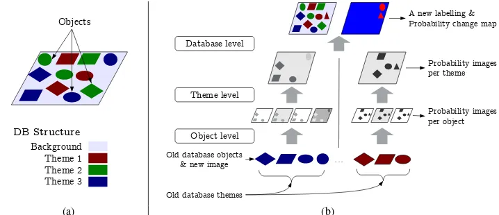
2.1.1 Inspection principle 2D geographical databases (DB) are structured in three different levels: a DB is composed of non-overlapping themes, and themes are themselves composed of ob-jects, that are in practice 2D polygons (cf. Figure 1a). Therefore, this hierarchical layout exhibits three levels of possible examina-tion: (1) the object level, (2) the theme level, and (3) the DB level. The initial DB is resampled at a resolution consistent with both the geometrical accuracy of its themes and the spatial resolution of the satellite image. Here, 1 m is selected as the most appro-priate scale of analysis. Since no overlapping themes exist in a DB, a pixel of such a grid can include not more than one label, corresponding to the theme of the object intersecting such pixel. Our methodology is based on such hierarchical inspection, in a ”bottom-up” way. Our method first performs a classification per each object of the database. Then, labels are merged at the theme level, and the final decision is taken at the DB level (Figure 1b). The object level inspection consists (1) in choosing, for each ob-ject, a subset of pixels that best allows to discriminate the object from the rest of the image (called hereoutside), and (2) in classi-fying the full image into two labels (inside/outside). The subset selection is based on the maximization of the recall a two-class classification of the pixels of the object (Section 2.1.2). There-after, the labelling process allows to obtain a probability map for each object of each theme of the database.
All classifications computed at the object level are then merged at the theme level, in order to obtain a single probability map per theme. This map describes the probability of each pixel of the image to belong to the current theme. Thanks to the object level inspection, the several existing visual aspects of the theme are
kept and no specific ones are favored (e.g., ones of the largest ob-jects).
Finally, a decision is taken at the DB level. A new label image is first produced, that associates to each pixel one label of the ini-tial DB. Secondly, a final probability change map is generated, allowing to label each pixel of the DB image aschangedornot changed, and to detectconfusion areas. This indicates where our method cannot straightforwardly take a decision. The reduction of those confusing areas will be the purpose of our next research.
2.1.2 Notations
Database A 2D geographical database is structured in several themes{Tj}j∈[1,NT], NT being the number of themes
(Equa-tion 1). Each themeTj is itself composed of a set of objects
{Oij}i∈[1,NTj],NTj being the number of objects of the themeTj
(see Figure 1a and Equation 2).
DB= [ j∈[1,NT]
Tj, (1)
∀j∈[1, NT], Tj= [ i∈[1,NTj]
Oij. (2)
Projection onto the image Each objectOji of the themeTjis associated to a regionRji of the image, by a projection function
I, given in Equation 3. Thus, each regionRji is a set of pixels of the image. Thereafter, objectOijand its image projectionRji will be noted equally, and the notationOjiwill be used.
∀j∈[1, NT], ∀i∈[1, NTj], R
j i=I(O
j
i). (3)
Moreover, when no ambiguity is possible, an objectOijand its associated themeTj will be notedOandT. The projection of all the objects composing a DB may not necessary cover the full area of the region of interestΩ: the rest of the area is denoted backgroundhereafter:
Ω =PI(DB)∪background.
Finally, each pixel of the image is initially labelled either by a theme of the DB either by being in thebackground({Bg}). The label of a pixelpof the imageIis given by the functionLas:
LDB:I −→ {Tj}j∈[1..NT]∪ {Bg}
p 7−→ LDB(p)
Classification Changes between the DB and the satellite image are assumed to be limited so that DB can be used to learn the visual aspect of existing objects, and therefore themes. Thus, DB objects are used to train the classifier, introduced in Sec. 2.3. Moreover, the training step is performed according to a subset of pixelsE, labelled in two classes{l1, l2}, with the functionl (Equation 4). {E, l}is called the training set, and can also be noted(E1, E2), whereE1 = {p ∈ E, l(p) = l1}andE2 =
{p∈E, l(p) =l2}.
l:E −→ {l1, l2} p 7−→ l(p)
From the training set{E, l}, the classification method allows to define a classification functionlc, that is applied to the full image:
lc:I −→ {l1, l2} p 7−→ lc(p)
A probability measure is derived from the classification, this mea-sure is defined as the probability of each pixel of the image to be-long to the classl1,P(lc(p) =l1), the probability to belong tol2 being equal to1−P(lc(p) =l1). Finally, a map of probabilities
Objects
Figure 1: (a) Database structure and (b) our hierarchical inspection methodology.
P(E, l) =P(E1, E2) :I −→ [0,1] p 7−→ P(lc(p) =l1)
Thereafter, the recall of a classificationlc, with regard to a ground-truthGT={EGT, lGT}(a subset of pixels whose label is known a priori), is defined as the number of pixels ofEGTthat are cor-rectly labelled bylc:
Recall(lc,GT) =Card(p∈EGT, lc(p) =lGT(p)).
2.2 The hierarchical process
The three levels of our inspection method are detailed thereafter. 2.2.1 Object level The object level inspection is based on a supervised classifier that is fed with a set of image-based features, described in Section 2.3. For each object, a specific classifier is trained on the subset of pixels, taken inside the object, able to best discriminate the object from the rest of the pixels of the image and out of the current theme. The selection of such a training set also allows to reduce registration issues between DB and images that is often reported in the literature (Poulain et al., 2009).
Training set selection The purpose of this part is to chose two pixels sets for appropriate training: one in the objectOof the themeT(SinO∗ ⊂O), and one out of the current theme (S two subsets are selected among several randomly generated sub-sets, as the subsets that maximise the recall of the classification (theme / out of theme). Such selection is performed in two steps: (1) the selection of the bestinsidesubset, and (2) the selection of the bestoutsidesubset.
First, theinsidesubset is selected as follows: a subset ofoutside pixels is randomly drawn within pixels out of the current object, Sout
O ⊂I\PI(T). Those pixels can belong to another theme or to thebackground. Then,Nininsidepixels are randomly drawn within pixels of the current object:
{Sinj
O }j∈[1..Nin]⊂O
Nin.
One classification is obtained per eachinsidesubset, paired with theoutsideone,{linj
c }j∈[1..Nin]. The recall of each classifier is
computed by using object pixels as ground-truth,GT={PI(O), l}. Theinsidesubset with the best recall is selected according to:
in∗= arg max j∈[1..Nin]
Recall(linj
c ,GT).
Secondly, theoutsidesubset is selected in the same way. Nout outsidesubsets are randomly drawn, and the corresponding clas-sifiers{loutj
Finally, the training set is defined as the union of the bestinside subsetSOin∗and the bestoutsideoneSout
Classification The optimal training subset SO∗, associated to the objectOis then used to perform a classification and to re-trieve a probability mapPO:
PO=P(SO) =∗ P(Si
∗
O, S e∗
O).
2.2.2 Theme level The probability mapsPO, computed for each objectOof a given themeT, are merged in order to obtain a single probability map per themePT
:
PT =Fusion({PO, O∈T}). (5)
For now, three merging methods have been tested, the minimal, the maximal and the weighted mean value. In this paper, the mean weighted by the size of the objects is used, in order to give more confidence in the larger objects, that are less likely to change. However, merging probability maps with Bayes rules is planed.
2.2.3 Database level For each pixel, the set of probabilities to belong to each theme{PT}
T∈DBis used to obtain the final label, corresponding to one of the theme, and a confidence map of such a labelling. Then, a final change map is computed by merging (1) the difference between the initial DB and the new classification, and (2) the confidence map.
Labelling and confidence map The final labellingLC1is
ob-tained by keeping, for each pixel, the theme with the highest prob-ability value. It is defined as follows:
LC1 :I −→ [1..NT]
p 7−→ arg max j∈[1..NT]
PTj(p)
A confidence valueCis associated with the classificationLC1. It
allows not to limit the system to a binary decision and to enhance confusion areas, i.e., areas where no straightforward decision can be taken. In practice, the maximal value of the probabilities of each theme provides a reliable measure of the confidence in the previous labelling:
Cmax:I −→ [0,1]
p 7−→ PTLC1(p)(p)
However, if two themes have both a high probability value, the maximum value is indeed high but the confidence should be low. Thus, amargingmeasure is preferred. It is defined as the dif-ference between the two highest probability values, related to LC1andLC2:
Cmargin:I −→ [0,1]
p 7−→ PTLC1(p)
(p)− PTLC2(p)
whereLC2(p)is the theme with the second highest probability
value inp.
Probability change map A change map∆is obtained by com-paring new labels with the initial DB. Thus, each pixel can take, either the value -1 (change), either the value 1 (no change):
∀p∈I, ∆(p) =
−1 siLC1(p)6=LDB(p)
1 siLC1(p) =LDB(p)
This change map∆is then weighted by the confidence measure, in order to derive a final probability change mapΠsuch as:
∀p∈I, Π(p) = ∆(p)∗C(p).
This map is composed of three classes:certain change,certain no-change, anduncertain(i.e., confusion areas, see Equation 6). For that purpose, two thresholdsS1andS2are introduced. They should be tuned according to the quality result and the percentage of false alarms that is tolerated.
∀p∈I,
Such labelling allows to focus an operator either on change areas, either on confusion areas.
2.3 Technical choices
2.3.1 Classifier The classification method must be adapted to the different themes of the analysed DB. Thus, a supervised clas-sification is chosen. Moreover, such a method should (1) handle a very large numbers of features (>200), (2) have a high gener-alisation ability, and (3) be fast enough to perform as many clas-sifications as required. Consequently, a Support Vector Machine (SVM) method was chosen (Foody et al., 2006), with a standard Gaussian kernel (k(x1, x2) =C∗e−γkx1−x2k
2
, where(x1, x2) are two feature vector). A grid search method was applied to select the best hyper-parameters (C,γ) that maximise the cross-validation accuracy. Each SVM provides a binary classification, coupled with a probability estimate per theme (Wu et al., 2004). 2.3.2 Features Our methodology is based on the fact that the various visual aspects of each theme of the DB can be retrieved. Since the most relevant features for a specific theme cannot be known beforehand, and since we aim to deal with any kind of theme, a large number of features computed from the different channels of the image is therefore required. The quality of our workflow is highly dependent on those features. A large body of literature has dealt with geospatial image-based feature extraction (Lefebvre et al., 2008; Lienou and Campedel, 2009; Tokarczyk et al., 2012). Features can be (1) spectral (resulting from the combi-nation of the input spectral channels of the image), (2) geometri-cal (i.e., low-level primitives such as lines or keypoints), and (3) textural (describing the image behaviour in the neighbourhood of each pixel).
With a sub-metric image, a multi-scale observation may be use-ful. Indeed, a small neighbourhood will probably provide more homogeneous textures and best describes fine textures (e.g., for-est or fields), while large neighbourhood allows to better for-estimate complex textures as vineyard or aligned buildings, (Campedel et al., 2005).
2.4 Training point selection
The number of training points is tuned to 200 (100insideand 100 outside), and the numbers of random selectionsNinandNoutis set to 10. However, a quantitative study will be carried out to know the real sensitiveness of such parameters with respect to the themes, and the area of interest.
3 RESULTS ON LAND COVER DATASETS
Our method was first assessed on simulated data in order to be independent of the input feature set and ground-truth issues. In (Gressin et al., 2013), we demonstrated that our methodology was
not sensitive to various kinds of change, the ratio of change and the varying visual aspect of objects within a specific theme. In this paper, our method was applied on real 2D geographic DB and satellite images. One area of interest acquired with a satellite im-age is first described. Then, change detection results performed for two different DB are provided.
3.1 Area of interest
Our dataset covers a surface of 760km2in the Southern-West part of France. One acquisition of the Pleiades sensor in August 2012 is available. This acquisition is composed of two images: one panchromatic 0.5 m ortho-image, used to compute textural fea-tures and one four channels 2 m ortho-image, for spectral ones. Three geographic DB are available on this area: the first one cor-responds to the agricultural activities (crops, pastures, . . . , called Fieldafterwards), the second one to forests (tree species, hedges etc.), and the third one to buildings. From these DB, two scenar-ios were generated. First, a DB with three very specific and de-tailed themes is proposed (called hereafterdetailed DB): the Dou-glas fir closest forestclass, thebread wheatclass, and the build-ingclass. The two first themes represent two specific sub-themes of the two most populated themes of the area: Fieldand For-est. They were selected to assess the relevance of our method to the classification of ”unknown” classes (compared to thebuilding class that has been analysed through many approaches). More-over, our method allows to not separatebuildingclass into several roof material dependent subclasses as it traditionally carried out. Change detection results on this DB are shown in Section 3.3. Secondly, a more global, inhomogeneous, and therefore challeng-ing land-cover DB is generated (calledglobal DB). All classes of theFieldandForestdatabases are merged into two themes, re-spectively. Therefore, theFieldandForestthemes are composed of objects of varying visual aspects and sizes. Results on this DB are shown in Sec 3.4.
3.2 Computed features
First, spectral features were computed: they were derived from the red, green, blue and near-infrared channels available (e.g., NDVI, SAVI etc.), and were computed using the Orfeo-ToolBox library (Inglada and Christophe, 2009). Those twelve features are mainly useful to discriminate vegetation and water bodies. Then, one textural feature, namely the entropy of the histogram of gradient directions, was introduced in order to bring informa-tion about the structure of the texture around each pixel vicinity. It allows to best discriminate irregularly textured objects (such as forests) from featureless objects (as fields) (Trias-Sanz, 2006).Fi-nally, dense SIFT descriptors are computed, in a regular pixel grid of the image (every 4 pixels), with a Gaussian filter ofσ = 1.2 (van de Sande et al., 2010) which is the default value of the algo-rithm. Then, a Principal Component Analysis is performed so as to extract the ten (empirical value) eigenvectors associated to the ten highest eigenvalues, so as to keep only the most discrimina-tive information.
3.3 Detailed DB results
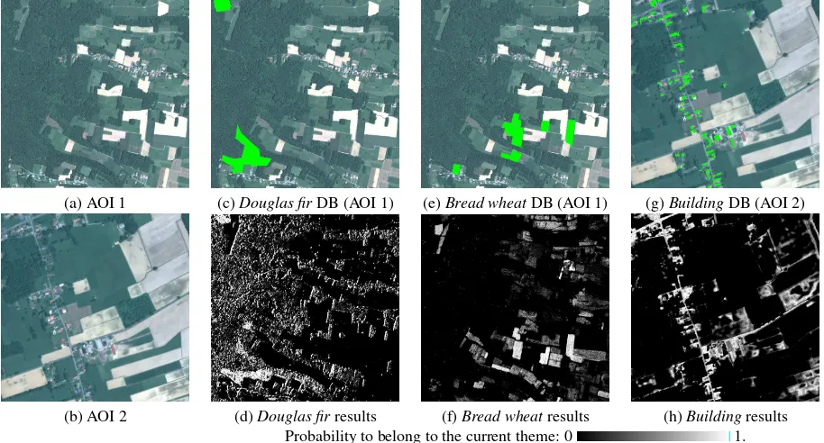
(a) AOI 1 (c)Douglas firDB (AOI 1) (e)Bread wheatDB (AOI 1) (g)BuildingDB (AOI 2)
(b) AOI 2 (d)Douglas firresults (f)Bread wheatresults (h)Buildingresults Probability to belong to the current theme: 0 1.
Figure 2: (a) and (b) The two specific areas of interest (AOI 1 and 2) of the Pl´eiades image. DB and the probability result at theme level for: (c) and (d) thedouglas firtheme (AOI 1), (e) and (f) thebread wheattheme (AOI 1), (g) and (h) thebuildingtheme (AOI 2). No DB fusion has been performed here.
method from founding new objects. Finally, the classification for thebuildingtheme is the most confusing. Indeed, our method is able to detect almost all existing and new buildings. However, the classification fails to discriminatebuildingfrom road, park lots, and dry parts of some fields, due to a restricted feature set (Fig-ures 2g and h).
These results do not take into account the DB fusion process, that would allow to reduce confusion between the existing themes of the DB.
3.4 Global DB result
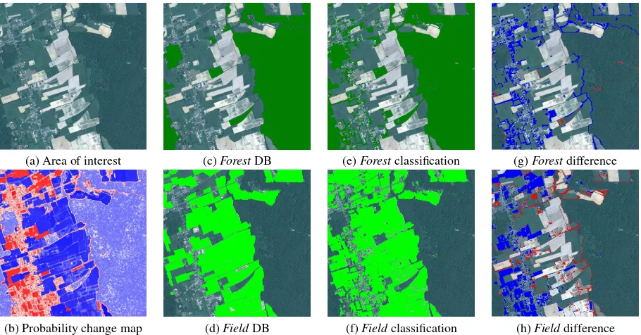
Finally, our change detection method was applied on theglobal DBscenario. This DB is composed of two themes, namelyField andForest. TheForesttheme is composed of 50 objects of vari-able sizes from 5 different forest themes, and theField theme gathers 190 objects from 20 different themes. Figure 3a and 3e show the area of interest and the final probability change map, re-spectively. One can notice extended red areas, corresponding to real changes on the ground, here new fields as well as forest dis-appearance or decrease. White areas are confusing areas, mainly objects that are not in the initial DB, like building, roads or other anthropic surfaces. These issues may be easily solved by intro-ducing more themes in our initial DB.
Changes can also be studied theme by theme. Thus, Figure 3 shows theForesttheme (b), the classification result after fusion at the DB level (c), and the differences between the DB and the classification (d). This change map enhances new areas (in blue) and disappeared areas (in red). Most disappearance correspond to clearings, not included in the DB. Blue areas are new forest areas, extended forest areas, as well as hedges and copses that are again not in the DB. Indeed, only objects larger that a minimal size are included in the DB. If necessary, the knowledge of such specification would allow us to filter such objects.
Moreover, Figure 3 also shows for theFieldDB (f), the classifi-cation result after fusion at the DB level (g), and the differences between both of them (h). This map shows many new fields (la-belled in blue) as well as removed ones (in red). Many field borders are labelled as disappeared. This is due to the coarse delineation ofFieldobjects during the initial image photointer-pretation process.
Finally, similarly to theDetailed DBscenario, no ground-truth is available and no qualitative assessment was possible. How-ever, visual inspection showed satisfactory results, allowing to correctly detect the main changes between the DB and the image.
4 CONCLUSION
In this paper, we proposed a classification-based method that al-lowed to obtain satisfactory change maps between unknown 2D land-cover databases and a more recent satellite image. Our hi-erarchical method was based on a carefully designed per-object training set selection and a generic decision fusion, guided by the database layout. As this process is independent of both the database specifications and the input image, it can be applied on a large number of real cases. Our classification and per-theme fu-sion processes were first assessed on three specific and challeng-ing themes. Despite a restricted number of features, our train-ing set selection allowed to deal with object disappearance, and correctly found new objects. Then, the change detection method-ology was applied on one land cover database composed of two very general themes (FieldandForest). We managed to find most changed areas. However, our method failed to discriminate some objects (as building from roads, or parking). Consequently, in future works, improvements of the method will focus on (1) the introduction of a large number of features, coupled with a feature selection step at the theme level and (2) a final regularization step at the DB level of the classifications obtained at the theme level.
References
Bovolo, F., Bruzzone, L. and King, R., 2013. Introduction to the special issue on analysis of multitemporal remote sensing data. IEEE TGRS 51(4), pp. 1867 – 1869.
Campedel, M., Moulines, E. and Datcu, M., 2005. Feature selec-tion for satellite image indexing. ESA-EUSC: Image Informa-tion Mining, Frascati Italy.
(a) Area of interest (c)ForestDB (e)Forestclassification (g)Forestdifference
(b) Probability change map (d)FieldDB (f)Fieldclassification (h)Fielddifference Figure 3: Results of the change detection method: (a) Orthoimage of the area of interest, (b) Probability change map (red: change – blue area: no change – white: confusing areas; (c)Foresttheme (d)Fieldtheme; (e) and (f) Classification results after DB fusion for theForestand theFieldthemes, respectively; (g) and (h) Differences between the DB and the classification (■: new areas and■ disappeared areas) for theForestand theFieldthemes, respectively.
Foody, G. M., Mathur, A., Sanchez-Hernandez, C. and Boyd, D. S., 2006. Training set size requirements for the classifi-cation of a specific class. RSE 104(1), pp. 1–14.
Gianinetto, M., 2008. Updating large scale topographic databases in Italian Urban areas with submeter QuickBird Images. IJNO 28(4), pp. 299–310.
Goyette, N., Jodoin, P., Porikli, F., Konrad, J. and Ishwar, P., 2012. Changedetection.net: A new change detection bench-mark dataset. In: Computer Vision and Pattern Recognition Workshops (CVPRW).
Gressin, A., Vincent, N. and Paparoditis, N., 2013. Semantic approach in image change detection. In: ACIVS.
Helmholz, P., Becker, C., Breitkopf, U., Buschenfeld, T., Busch, A., Braun, C., Grunreich, D., Muller, S., Ostermann, J. and Pahl, M., 2012. Semi-automatic Quality Control of Topo-graphic Data Sets. PE & RS 78(9), pp. 959–972.
Holland, D., Boyd, D. and Marshall, P., 2006. Updating topo-graphic mapping in Great Britain using imagery from high-resolution satellite sensors. ISPRS Journal of Photogrammetry and Remote Sensing 60(3), pp. 212–223.
Hussain, M., Chen, D., Cheng, A., Wei, H. and Stanley, D., 2013. Change detection from remotely sensed images: From pixel-based to object-based approaches. ISPRS Journal of Pho-togrammetry and Remote Sensing 80, pp. 91–106.
Inglada, J. and Christophe, E., 2009. The Orfeo Toolbox remote sensing image processing software. In: IGARSS, pp. 733–736.
Lefebvre, A., Corpetti, T. and Hubert-Moy, L., 2008. Object-oriented approach and texture analysis for change detection in very high resolution images. In: IGARSS, pp. 663–666.
Lienou, M. and Campedel, M., 2009. Image semantic coding using OTB. In: IGARSS, pp. 745–748.
Marc¸al, A., Borges, J., Gomes, J. and Pinto Da Costa, J., 2005. Land cover update by supervised classification of segmented ASTER images. IJRS 26(7), pp. 1347–1362.
Miller, O., Pikaz, A. and Averbuch, A., 2005. Objects based change detection in a pair of gray-level images. Pattern Recog-nition 38(11), pp. 1976–1992.
Nemmour, H. and Chibani, Y., 2006. Multiple support vector machines for land cover change detection: An application for mapping urban extensions. ISPRS Journal of Photogrammetry and Remote Sensing 61(2), pp. 125–133.
Petitjean, F., Inglada, J. and Gancarski, P., 2012. Satellite Im-age Time Series Analysis Under Time Warping. IEEE TGRS 50(8), pp. 3081–3095.
Poulain, V., Inglada, J., Spigai, M., Tourneret, J.-Y. and Marthon, P., 2009. Fusion of high resolution optical and SAR images with vector data bases for change detection. In: IGARSS, pp. 956–959.
Radke, R., Andra, S., Al-Kofahi, O. and Roysam, B., 2005. Im-age change detection algorithms: a systematic survey. IEEE Transactions on Image Processing 14(3), pp. 294–307.
Robin, A., Moisan, L. and Le H´egarat-Mascle, S., 2010. An a-contrario approach for subpixel change detection in satellite imagery. IEEE PAMI 32(11), pp. 1977–93.
Tokarczyk, P., Montoya, J. and Schindler, K., 2012. An eval-uation of feature learning methods for high resolution image classification. ISPRS Annals of the Photogrammetry, Remote Sensing and Spatial Information Sciences I-3, pp. 389–394.
Trias-Sanz, R., 2006. Texture Orientation and Period Estimator for Discriminating Between Forests, Orchards, Vineyards, and Tilled Fields. IEEE TGRS 44(10), pp. 2755–2760.
van de Sande, K., Gevers, T. and Snoek, C., 2010. Evaluating color descriptors for object and scene recognition. IEEE PAMI 32(9), pp. 1582–96.
Walter, V., 2004. Object-based classification of remote sensing data for change detection. ISPRS Journal of Photogrammetry and Remote Sensing 58(3-4), pp. 225–238.