Heuristic methods for cost-oriented assembly
line balancing: A survey
Matthias Amen
*
Institut fu(r Unternehmensrechnung und Controlling, University of Berne, Engehaldenstrasse 4, CH-3012 Bern, Switzerland
Received 17 March 1998; accepted 21 September 1998
Abstract
This paper is concerned with cost-oriented assembly line balancing. This problem occurs especially in the "nal assembly of automotives, consumer durables or personal computers, where production is still very labour-intensive, and where the wage rates depend on the requirements and quali"cations to ful"l the work. First a short problem description is presented. After that a classi"cation of existent and new heuristic methods for solving this problem is given. The heuristic methods presented in this paper are described in detail. A new priority rule called`best change of idle costais proposed. This priority rule di!ers from the existent priority rules because it is the only one which considers that production cost are the result of both, production time and cost rates. Furthermore a new sophisticated method called`exact solution of
sliding problem windowsais presented. The solution process is illustrated by an example, showing how this metaheuristic
works together with an exact method. ( 2000 Elsevier Science B.V. All rights reserved.
Keywords: Assembly line balancing; Cost-oriented production planning; Heuristic methods
1. Introduction
In anassembly linethe product units move with a constant transportation speed through the con-secutive stations. The total work content to be performed by the production system has been split up into economical indivisible work elements which are calledtasks. Among the set of tasks there existtechnological precedence relations. The set of tasks to be performed in the same station is called anoperationor astation load. The time to perform an operation is restricted by the cycle time. The
*Tel.:#41-31-631-85-01; fax:#41-31-631-37-80.
E-mail address:[email protected] (M. Amen)
assembly line balancing problem consists in al-locating the tasks to the stations subject to the technological precedence relations, the cycle time restriction of the stations and the indivisibility of the tasks.
In literature the objective usually is to minimize the number of stations in a line for a "xed cycle time [1, p. 650]. In other words: The objective is to minimize the total idle time of the total capacity provided by the sum of the stations of the line [2, p. 911]. Therefore, this is calledtime-oriented assem-bly line balancing. The objective in cost-oriented assembly line balancingwhich is considered in this paper isto minimize the total cost per product unit [3}6].
In general, assembly is a labour-intensive kind of production. Therefore, in cost-oriented assembly
line balancing, thelabour costhas to be analyzed in detail: The wage rate of each operation depends on the maximal point value of the tasks assigned to a station. As the tasks di!er in their di$culty, there are di!erences in the point values and thus in the corresponding wage rates. The worker has to be paid for the whole cycle time irrespective of the duration of the operation. So the total labour cost per product unit is the sum of the wage rates of all stations multiplied by the cycle time. Further it is assumed that the cost of capitaldepends on the overall line length and that all stations have the same length. All other costs (e.g. material cost) can be assumed to be indepen-dent of the division of labour and of the line length [3, p. 82]. Introducing the following symbols:
I number of tasks (!) i index for the tasks,i"1(1)I M number of stations (!)
m index for the stations,m"1(1)M
I4
m set of tasks, assigned to stationm,m"1(1)M c cycle time (TU/PU)
k total cost per unit (MU/PU)
k4
m cost rate of stationm,m"1(1)M(MU/TU) k43 cost of capital per station (MU/PU)
k48
(Note: Dimensions: TU, time units; PU, product units; MU, monetary units; Labels: r, cost of capi-tal; s, station; t, task; w, wage rate.)
Thetotal cost per product unitcan be calculated as
k"
A
+MSince the conveyor speed is "xed by the cycle time, the cost of capital for a single station can be transformed into a cost rate per time unit. The total cost of capital can be formulated as Mk43"cM(k43/c). Thus for the purpose of capacity balancing the relevant cost rates per time unit are made up by the sum of the capital cost per time unit and the task-depended wage rates:k5
i"k58i #k4#/c
andk4
m"k48m#k4#/c. This simpli"es the calculation
of the total cost per product unit to
k" +M
The total cost per product unit k"+M m/1ck4m
di!er from the term+Ii/1d5
ik5i only by the idle cost
per product unit which are caused by idle time and/or cost rate di!erences of the tasks assigned to the same station. Therefore, the objective to minim-ize the total cost per product unit is equivalent to minimize the total idle cost per product unit.
2. Classi5cation of heuristic methods for solving the cost-oriented assembly line balancing problem
As theNP-complete bin-packing problem can be reduced to the time-oriented assembly line balanc-ing problem in polynomial time, the time-oriented assembly line balancing problem is NP-hard [7, p. 56]. This also holds for the cost-oriented prob-lem [4, p. 479]. Thus it is justi"ed to develop heuristic solution methods.
There exist two di!erent general approaches for assembly line balancing. Inthe station-oriented ap-proachin each step of the solution process only one station is considered. Therefore we have to look for tasks which have to be assigned to the current station. Inthe task-oriented approachin each step of the solution process a selected task is considered. Therefore we have to look for the station to which the current task has to be assigned to [8, pp. 917}918; 9, pp. 182}184]. All of the methods de-scribed in this paper use the station-oriented ap-proach. Fig. 1 gives an overview of the existent and new methods which can be classi"ed as follows:
Most of the methods can be characterized as random choice/priority rule methods. In each step of the solution process all of the methods of this category but one choose one of alternative tasks for assignment. For determining the task either ran-dom choice or priority rules are used. The priority rule methods can be distinguished into methods that make use of one problem-oriented priority rule and methods that use several problem-oriented priority rules. Priority rules are called problem-oriented if they consider structural aspects of the
Fig. 1. Heuristic methods for cost-oriented assembly line balancing.
problem. The set of problem-oriented priority rules consists of three subclasses.The time-oriented prior-ity rules consider only the durations and/or the precedence relations of the tasks, the cost rate-oriented priority rulesconsider only the cost rates of the tasks. Due to the fact that cost are the product of both, cost-rate and duration, the new cost-oriented priority rule **best change of idle cost++
which will be presented in the next section takes both aspects into account. In methods with several problem-oriented priority rules the single rules are used in lexicographic order, i.e. problem-oriented priority rules are used as tie-breakers. All priority rule methods use a simple non-problem-oriented priority rule as a"nal tie-breaker.
One priority method di!ers from the other as in the major steps of the solution process one of sev-eral alternative station loads has to be chosen by the use of di!erent priority rules which consider the situation in the alternative station loads. The alter-native station loads are generated by the use of several problem-oriented priority rules to choose one of alternative tasks. Thus this method is a further development of the previous mentioned methods.
The new method called**exact solution of sliding problem windows++ is quite di!erent from the tic methods mentioned before because it is a heuris-tic version of an exact method. With respect to the similarities of the heuristic methods, the methods are grouped into the following classes:
f Z methods with random choice task assignment; f P methods with one problem-oriented priority
rule;
f H methods with several problem-oriented prior-ity rules;
f F methods with exact solution of sliding problem windows;
f E exact method.
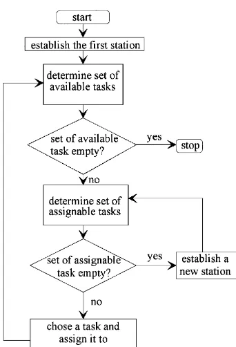
Fig. 2. Procedure for assigning tasks to stations.
this method is not presented in this paper (for further reading see [5,6]. The exact method works as a subalgorithm for the methods of class F.
3. Methods with choice of one of alternative tasks
All methods with choice of one of alternative tasks in each step of the solution process follow the same procedure when assigning tasks to stations. The procedure is shown in Fig. 2.
As the station loads are generated successively, in each step of the procedure only one station is con-sidered (station-oriented approach). The tasks which have no predecessor task or only predecessor tasks already assigned to the current or to an earlier station are called available. The available tasks which have a duration not longer than the remain-ing idle time of the considered station are called assignable. Among the set of assignable tasks one task is chosen according to the method used. After assigning this task the sets of available and assign-able tasks are updated immediately. If the set of
assignable tasks is empty, the current station is **maximally loaded++ [10, p. 266; 8, p. 918]. Then a new station is established and the set of assignable tasks has to be updated again. Each method stops after all tasks have been assigned to a station.
The random choice method (class Z) [11, pp. 25}35 and 44}46] can be used several times for solving the same problem instance. Among the set of randomly generated solutions for the same prob-lem instance only the best one has to be considered for realization.
For a formal description of the priority rule methods, the following additional symbols are in-troduced:
I!44*'/ set of assignable tasks
d5
i duration of taski, i"1(1)I(TU/PU) F
i set of all technological immediate followingtasks of taski, i"1(1)I *k
i change of idle cost if taskto the currently considered station,iwill be assignedi3I!44*'/
(MU/PU) r
i ranked positional weight of task(TU/PU) i,i"1(1)I
With this symbols the following problem-oriented priority rulesof classPcan be de"ned:
z P-MaxD Maximal task duration [12, p. 728],
i.e. maxMd5
iDi3I!44*'/N.
z P-MaxR Maximal ranked positional weight
([13, p. 395 in the modi"ed version
z P-MaxF Maximal number of immediate
followers [12, p. 728], i.e. maxMDF
iD Di3I!44*'/N.
z P-MaxKt Maximal cost rate [4, p. 481], i.e.
maxMk5
iDi3I!44*'/N.
z P-MinKt Minimal cost rate [3, pp. 106}107],
i.e. minMk5
iDi3I!44*'/N.
z P-MinKts Minimal absolute di!erence to the
current station cost rate [3, pp. 106}107], i.e. minMDk5
i!k4mD Di3I!44*'/N.
Fig. 3. Calculation of*k
i.
z P-MinKI Best change of idle cost, i.e.
minM*k
The non-problem-oriented priority rule
z P-MinI Minimal task number [12, p. 729],
i.e. min MiDi3I!44*'/N (Usually the tasks are numbered topologically ac-cording to the precedence relations.)
is used as "nal tie breaker in all priority rule methods. While applying the new priority rule`best change of idle costa(P-MinKI) both decreases and increases can occur, which has to be accepted. Not choosing an assignable task with *k
i'0 and
es-tablishing a new station in some cases may cause an extra station and therefore higher overall idle cost. The calculation of*k
i is illustrated in Fig. 3.
P-MinKts and P-MinKI are dynamic rules be-cause they depend on the current cost rate of the station. For these rules it is necessary to calculate not only the remaining idle time of the current station after each assignment, but also to update the cost rate of the station immediately. While P-MaxD, P-MaxR and P-MaxF are only time-oriented and P-MaxKt, P-MinKt and P-MinKts depend only on the cost rates, P-MinKI is the only priority rule which considers that cost results from
both, the cost rates and the time needed by the workers of the line.
Within class H there exist three priority rule methods with the choice of one of alternative tasks in each step of the procedure. The lexicographic orders of priority rules of these heuristic methods are given below. For the heuristic methods of Stef-fen and Heizmann the lexicographic order di!ers according to the fact whether the station is just established (empty station) or the station has been established at an earlier step in the solution process (partially"lled station).
z H-Stef Heuristic method of Ste!en [3, pp.
105}110]: Lexicographic order of priority rules in case of just established stations (station is empty):
Lexicographic order of priority rules in case of already established stations (station is partially
"lled with tasks):
1. P-MaxR 1. P-MinKts
2. P-MinI 2. P-MinKt
3. P-MaxR 4. P-MinI
z H-Heiz Heuristic method of Heizmann [15,
pp. 110}124]: Lexicographic order of priority rules in case of just established stations (station is empty):
Lexicographic order of priority rules in case of already established stations (station is partially
"lled with tasks): 1. P-MaxD 1. Identity of task
cost rate and current station cost rate (i.e. Dk5
i!k4mD"0 is
required).
2. P-MinI 2. P-MaxD
3. P-MinI
z H-WR Heuristic method`wage rateaof
Rosen-berg/Ziegler [4, p. 481]: 1. P-MaxKt
2. P-MaxD 3. P-MinI
This heuristic method is a modi"cation of the well-known `"rst-"t decreasing heighta-method suggested for solving two-dimensional packing problems [16, p. 810]. The method is called `wage ratea because Rosenberg/Ziegler [4] consider only labour cost.
4. A method with choice of one of alternative station loads
A priority-rule method with choice of one of alternative station loads is the`wage rate smooth-inga method (H-WRS) [4, pp. 481}484]. The method consists of a three-phase algorithm. In order to give a formal description of this method the following symbols are introduced:
I3%45 set of not yet"nally assigned tasks I4,105,1)!4%2
m set of tasks which destation load of station"nes the potentialm in phase 2, m"1(1)M
I4,105,1)!4%3
m set of tasks which destation load of station"nes the potentialm in phase 3, m"1(1)M
= number of di!erent cost rates (!) w index of the cost rate,w3M1,2,=N I!44*'/,l
w set of assignable tasks with the costratekl
w,w"1(1)= ;
w number of potential station loads forthe currently considered task cost rate
kl
w(!),w"1(1)=
u index of the potential station loads,
u3M1,2,;
wN
I4,,,105
m,w,u set of tasks which detential station load for the considered"nes the uth
po-cost rate kl
m,w,u set of tasks which detial station load for the considered cost"nes theuth
poten-ratekl
are assignable to station m if the current station load is de"ned by the set of tasks I4,,,105
"xed variable which indicates in phase 1 whether phase 1 has to be restarted or whether phase 2 has to be started (!)
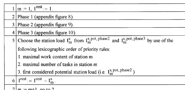
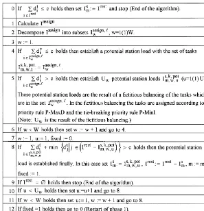
Fig. 4 shows the major steps of the 3-phase algorithm. The formal descriptions of the phases 1}3 are given in the appendix.
In phase 1 of the procedure, potential station loads are established. In phases 2 and 3 the poten-tial station loads which have been calculated in phase 1 are taken and further tasks are assigned. In phase 1 each potential station load consists only of tasks which have identical cost rates. The phases 2 and 3 are completely separated from each other. In phase 2 a potential station load taken from phase 1 is"lled further only with tasks which have the same cost rate as the station cost rate. In phase 3 a poten-tial station load taken from phase 1 is"lled further with tasks which could have cost rates di!erent from the station cost rate of phase 1. In step 5 a sta-tion load has to be chosen from the two alternative station loads which have been obtained from the phases 2 and 3. After a potential station load is
"nally"xed, in step 5 the algorithm moves back to phase 1. Within phase 1 stopping-criteria are to be checked at two di!erent steps.
5. A method with exact solution of sliding problem windows
A new heuristic method which is quite di!erent from those described in the foregoing sections is the `exact solution of sliding problem windowsa(class F). This heuristic is an application of the`working
Fig. 4. Wage rate smoothing.
forward techniquea[17, pp. 315}316]. The key con-cept is to solve consecutive small problems by the use of an exact method. A part of the optimal solution of a small problem will be "xed "nally. Then the next small problem will be de"ned and solved optimally. This process continues until the last small problem is solved. Similar methods for solving di!erent assembly line balancing problems were suggested in [18}20].
The idea to develop a heuristic application of an exact method derives from the fact that all existent heuristic methods load the stations maximally, but thatthe cost-oriented optimal solution could be mis-sedif the stations are"lled in this way [5, p. 225; 6, 1998a]. The exact method used is the only existent method in which the stations are not necessarily loaded maximally.
5.1. Formal description of the method
For a formal description of the`exact solution of sliding problem windowsathe following additional symbols are introduced:
I18 maximal number of tasks in a problem window (!)
I1!35 set of tasks which are in a problem win-dow
M,6. number of the currently "nally estab-lished stations (!)
M1!35 number of stations which are needed in the solution of a problem window (!)
M&*9 number of stations which are needed in the solution of a problem window and which are"nally established (!)
PartM proportion of the maximal number of
"nally established stations to the number of stations which are needed in the solu-tion of a problem window (!).
An important assumption for the formal descrip-tion which is given in Fig. 5 is the topological numberingof the tasks, i.e. ifi3F
hthenh(iholds.
If the tasks are not numbered topologically then they have to be renumbered"rst.
Fig. 5. Exact solution of sliding problem windows.
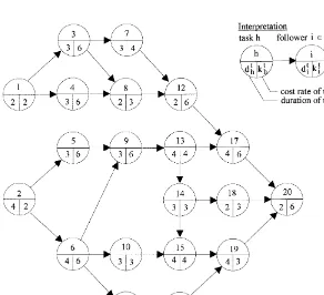
Fig. 6. Precedence graph for the example (cycle timec"10 TU/PU).
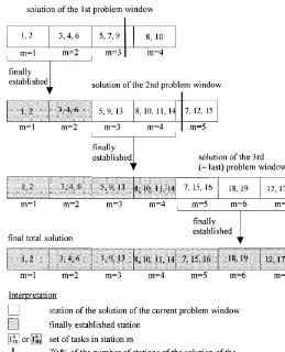
Fig. 7. Illustration of the exact solution of sliding problem windows.
Table 1
Optimal solution of the 1st problem window Station
m
Station load
Duration of the operation
Cost rate of the station I4
m dm4 k4m
(TU/PU) (MU/TU)
1 M1, 2N 6 2
2 M3, 4, 6N 10 6
3 M5, 7, 9N 9 6
4 M8, 10N 5 3
M1!35": 4 stations were needed to perform the tasks 1}10. According to the formulaM&*9:"maxM1,xPartM)M1!35yNwe establish "nally M&*9": maxM1,x0.7)4yN"maxM1,x2.8yN"2 stations. The tasks 1 and 2 are"nally assigned to station 1, the tasks 3, 4 and 6 are"nally assigned to station 2. The assignments of tasks to the stations 3 and 4 are abolished.
Table 2
Optimal solution of the 2nd problem window Station
m
Station load
Duration of the operation
Cost rate of the station I4
m d4m k4m
(TU/PU) (MU/TU)
1 M5, 9, 13N 10 6
4 M8, 10, 11, 14N 10 3
5 M7, 12, 15N 9 6
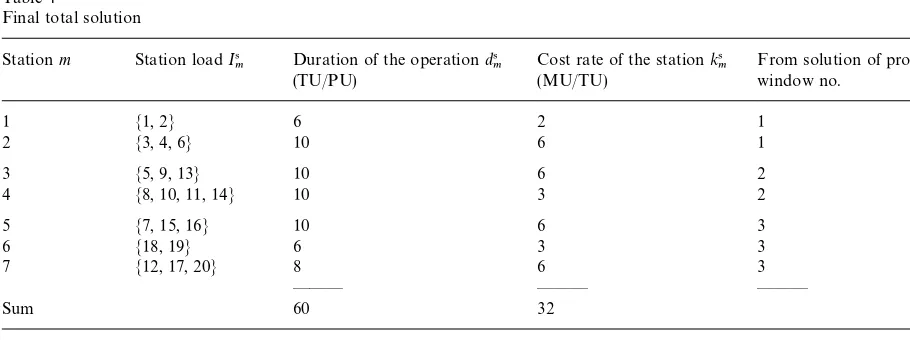
Table 4
Final total solution
Stationm Station loadI4
m Duration of the operation(TU/PU) d4m Cost rate of the station(MU/TU) k4m From solution of problemwindow no.
1 M1, 2N 6 2 1
Optimal solution of the 3rd problem window Station
M1!35:"3 stations were needed to perform the set of tasks in this last problem windowI1!35. Because this is the last problem window we establish"nally allM1!35stations. The tasks 7, 15 and 16 are"nally assigned to station 5, the tasks 18 and 19 are
"nally assigned to station 6, the tasks 12, 17 and 20 are"nally assigned to station 7.
same problem window, which otherwise may occur according to the parameter constellations, we have to ensure that at least one station of the solution is established "nally. Therefore we set M&*9"max: M1,xPartM)M1!35yN. The tasks assignments of the M1!35}M&*9 last stations of a solution of a problem window are abolished. In the next problem window a balance for the IPWlowest numbered not yet assigned tasks has to be generated and the"rstM&*9stations have to be "nally established. This procedure continues until allItasks are"nally assigned to a station.
5.2. An example of the solution process
The method described in Section 5.1 will now be illustrated by an example. Fig. 6 shows the preced-ence graph of the problem instance together with the durations and the cost rates of the tasks. A pre-cedence graphG"(M1,2,IN,R) consists of the set of tasks M1,2,IN and the set of precedence rela-tionsR. A precedence relation with ias technolo-gical immediate follower ofh,i3F
h, is illustrated by
an arrow (h,i) which is directed from h to i [21, p. 685]. The cycle time for this instance is given by c"10 TU/PU. Note that the tasks of the instance are numbered topologically.
The 20-task-instance will be solved by a version of the method which works with a maximum of IPW"10 tasks in each problem window. From a solution of a problem window about 70% of the station loads generated were"nally established, i.e.
PartM"0.7.
In our implementation of this method we used theexact backtracking methodsuggested by Amen [5,6]*this is the only existent method to generate an optimal solution for a cost-oriented assembly line balancing instance. The initial upper bound for the minimum cost per product unit which is needed in this exact method was obtained from the heuristic solution of the problem window by the use of the new priority rule`best change of idle costa(P-MinKI).
Fig. 8. Phase 1 of wage rate smoothing.
Fig. 7 gives a comprehensive illustration of the solution process for this example. As the exact method is beyond the topic of this paper the enumeration process and the dominance criteria of this backtracking-procedure are not explained here. In fact even for the solution of the"rst prob-lem window with 10 task approximately 100 iter-ations were needed. Because to give detailed information on the exact method is much space-and time-consuming, it is left for further reading (see [5,6]).
(1) Dexnition and solution of the xrst problem window. The"rst problem window consists of the
"rst IPA"10 lowest numbered (not yet "nally assigned) tasks. These are the tasks 1}10. Using the exact method we get the solution shown in Table 1.
(2) Dexnition and solution of the second problem window.First we have to calculate the set of not yet
"nally assigned tasksI3%45. These are the tasks 5 and 7}20. The "rst IPA"10 lowest numbered task among the setI3%45are taken into the set of tasks of this problem window I1!35. Therefore, we get I1!35": M5, 7, 8, 9, 10, 11, 12, 13, 14, 15N. Again, we solve this problem window with the exact method and calculate the solution shown in Table 2.
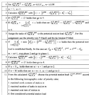
Fig. 9. Phase 2 of wage rate smoothing.
exact method and obtain the solution shown in Table 3.
(4) Final total solution.Combining the"nal assign-ments which are calculated in the solutions of the problem windows we get the "nal total solution (Table 4).
As the minimum cost is 310 MU/PU, the solu-tion generated by this method has the second lowest possible cost (320 MU/PU). To give addi-tional information we have found that there exist 18 optimal solutions for this problem instance. In each of the optimal solutions 7 stations were needed. The lowest realizable number of stations is 6 (94 solutions). With 6 stations a minimum of 330 MU/PU for the cost is calculated. Note that the stations 1 and 6 are not loaded maximally. This is another evidence that loading the stations
maxi-mally could prevent one from generating low-cost solutions [5, p. 225; 6].
6. Summary and outlook
This paper is concerned with the existent and new heuristic methods for solving the cost-oriented assembly line balancing problem. The methods are classi"ed and described in detail. Two new heuristic methods are presented: The priority rule `best change of idle costa and the more sophisticated method`exact solution of sliding problem windowsa. The sliding problem window technique is a new class of its own. It can be taken as ametaheuristic because its possible application is not only for the assembly line balancing, but also for some other problems with precedence relations. In a further
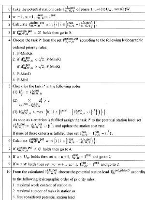
Fig. 10. Phase 3 of wage rate smoothing.
paper a comparison of the heuristic methods ac-cording to the solution quality and the computing time is presented [22].
Appendix
The formal discriptions of the phases 1}3 are given in Figs. 8}10.
References
[1] S. Ghosh, R.J. Gagnon, A comprehensive literature review and analysis of the design, balancing and scheduling of assembly systems, International Journal of Operations Research 27 (1989) 637}670.
[2] I. Baybars, A survey of exact algorithms for the simple assembly line balancing problem, Management Science 32 (1986) 909}932.
[4] O. Rosenberg, H. Ziegler, A comparison of heuristic algo-rithms for cost-oriented assembly line balancing, Zeit-schrift fuKr Operations Research 36 (1992) 477}495. [5] M. Amen, Ein exaktes Verfahren zur kostenorientierten
Flie{bandabstimmung, in: U. Zimmermann et al., (Eds.), Operations Research Proceedings 1996, Springer, Berlin, 1997, pp. 224}229.
[6] M. Amen, An exact method for cost-oriented assembly line balancing, International Journal of Production Economics 64 (2000) 187}195.
[7] T.S. Wee, M.J. Magazine, Assembly line balancing as gen-eralized bin packing, Operations Research Letters 1 (1982) 56}58.
[8] St.T. Hackman, H.J. Magazine, T.S. Wee, Fast, e!ective algorithms for simple assembly line balancing problems, Operations Research 37 (1989) 916}924.
[9] A. Scholl, Balancing and Sequencing of Assembly Lines, 2nd ed., Physica-Verlag, Heidelberg, 1999.
[10] J.R. Jackson, A computing procedure for a line balancing problem, Management Science 2 (1956) 261}271. [11] F.N. Silverman, The e!ects of stochastic work times on the
assembly line balancing problem, Ph.D. Thesis, Columbia University, New York, 1974.
[12] F.M. Tonge, Assembly line balancing using probabilistic combinations of heuristics, Management Science 11 (1965) 727}735.
[13] W.B. Helgeson, D.P. Birnie, Assembly line balancing using the ranked positional weight technique, Journal of Indus-trial Engineering 12 (1961) 394}398.
[14] R. Hahn, Produktionsplanung bei Linienfertigung, Walter de Gruyter, Berlin, 1972.
[15] Heizmann, J., Soziotechnologische Ablaufplanung verketteter Fertigungsnester zur ErhoKhung der FlexibilitaKt von Mon-tage-Flie{linien, Jochem Heizmann Verlag, Karlsruhe, 1981. [16] E.G. Co!man et al., Performance bounds for level-oriented two-dimensional packing algorithms, SIAM Journal on Computing 9 (1980) 808}826.
[17] C. Imboden, A. Leibundgut, P. Siegenthaler, Klassi" ka-tion heuristischer Prinzipien: Ein methodologischer Beit-rag zur Entwicklung von heuristischen Verfahren, Die Unternehmung 32 (1978) 295}330.
[18] L.B.J.M. Sturm, An improved method for balancing as-sembly lines, Working paper R 70/1, Interfaculty for Grad-uate Studies in Management, Rotterdam, 1970.
[19] W.H. Thomas, N.R. Reeve, Balancing continuous stochas-tic assembly lines, in: American Institute of Industrial Engineers, Technical Papers, 23rd Annual Conference and Convention of the American Institute of Industrial Engin-eers, Anaheim, California, 1972, pp. 409}419.
[20] N.R. Reeve, W.H. Thomas, Balancing stochastic assembly lines, AIIE [American Institute of Industrial Engineers] Transactions 5 (1973) 223}229.
[21] R. Reiter, On assembly-line balancing problems, Opera-tions Research 17 (1969) 685}700.
[22] M. Amen, Heuristic methods for cost-oriented assembly line balancing: A comparison on solution quality and computing time, International Journal of Production Economics 69 (2001) Forthcoming.