TEORI PENGAMBILAN KEPUTUSAN

(1)

TEORI PENGAMBILAN

KEPUTUSAN

(2)

D i i

A l i

Decision Analysis

Model yang membantu para manajer memperoleh

pengertian dan pemahaman yang mendalam, tetapi

mereka tidak dapat membuat keputusan.

Pengambilan keputusan merupakan suatu tugas

lit d l

k it

d

yang sulit dalam kaitan dengan:

(3)

Deciding Between Job Offers

Perusahaan A

• Suatu industri baru yang bisa memperoleh keuntungan yang tinggi • Suatu industri baru yang bisa memperoleh keuntungan yang tinggi

(booming)

• Gaji awal yang rendah, tetapi bisa meningkat dengan cepat. • Terletak dekat teman, keluarga dan team olah raga favorit

Perusahaan B Perusahaan B

• Perusahaan yang dibentuk dengan kekuatan keuangan dan komitmen pada karyawan.

• Gaji awal lebih tinggi tetapi kesempatan kemajuan lambat.

• Penempatan mendalam, menawarkan budaya.atau aktivitas olahraga

(4)

Keputusan terbaik vs Hasil terbaik

• Pendekaan struktur pengambilan keputusan dapatPendekaan struktur pengambilan keputusan dapat

membantu membuat keputusan yang terbaik, tetapi tidak dapat menggaransi hasil yang baik. p gg y g

• Keputusan yang barik kadang-kkadasng menghasilkan hasil yang kurang baik.

(5)

Bagaimana membuat keputusan

dalam organisasi

¾

Membuat keputusan:

h f h i f i f d li i h

– The process of choosing a course of action for dealing with a problem or opportunity.

(6)

Bagaimana membuat keputusan

dalam organisasi

k h l k h d l b k ik

¾ Langkah-langkah dalam membuat keputusan semantik.

– Menggambarkan dan mengenali masalah dan kesempatan. – Mengidentifikasi dan menganalisis macam langkah tindakan

alternatif, mengestimasi pengaruhnya dalam masalah atau kkesempatan.

(7)

Bagaimana keputusan dibuat dalam

organisasi?

• Proses pengambilan keputusan sistematis tidak

mungkin diikuti jika perubahan substansiil yang

terjadi dan banyak teknologi baru yang digunakan

terjadi dan banyak teknologi baru yang digunakan.

• Teknik keputusan novel boleh menghasilkan

pencapaian atasan dalam situasi tertentu

pencapaian atasan dalam situasi tertentu.

• Konsekwensi pengambilan keputusan yang etis harus

dipertimbangkan

(8)

Bagaimana keputusan di ambil dalam

organisasi?

Lingkungan keputusan meliputi:

• Lingkungan tertentu.

• Mengambil resiko lingkungan.

• Lingkungan tidak-pasti.

(9)

Bagaimana keputusan dibuat dalam

organisasi

?

¾

Lingkungan tertentu

¾

Lingkungan tertentu.

– Bilamana informasi adalah cukup untuk

meramalkan hasil dari tiap alternatif dalam

pengambangan implementasi.

– Kepastian adalah masalah ideal dalam

Kepastian adalah masalah ideal dalam

memecahkan dan pengambilan keputusan

lingkungan.

(10)

Bagaimana keputusan dibuat dalam

organisasi

?

¾

Resiko lingkungan

¾

Resiko lingkungan.

– Bilamana pembuat keputusan tidak dapat menyudahi

kepastian mengenai hasil berbagai macam tindakan, tetapip g g , p mereka dapat merumuskan kemungkinan kejadian.

– Kemungkinan dapat dirumuskan melalui sasaran prosedur i ik i i i ib di

(11)

Bagaimana keputusan dibuat dalam

organisasi

?

¾ Lingkungan ketidak-pastian.

– Bilamana manager memiliki sedikit informasi bahwa mereka tidak dapat menetapkan kemungkinan suatu kegiatan dari berbagai alternatif dan kemungkinan hasil.

– Ketidak-pastian memaksa pembuat keputusan bersandar pada individu dan kreativitas kelompok untuk berhasil dalam memecahkan masalah. – Juga yang ditandai oleh dengan cepat mengubah:g y g g p g

• Kondisi-Kondisi eksternal.

• Kebutuhan teknologi informasi.

• Personil yang mempengaruhi definisi pilihan dan masalah • Personil yang mempengaruhi definisi pilihan dan masalah. – perubahan yang cepat ini adalah juga disebut anarki terorganisir.

(12)

Bagaimana keputusan dibuat dalam

organisasi

?

¾ Bentuk-bentuk keputusan.p

– Keputusan terprogram.

• Melibatkan permasalahan rutin yang muncul secaraMelibatkan permasalahan rutin yang muncul secara

teratur dan dapat ditujukan melalui tanggapan standard. – Keputusan tidak terprogram.Keputusan tidak terprogram.

• Melibatkan bukan permasalahan rutin yang

(13)

Teori Pengambilan Keputusan

Pola dasar berpikir dlm konteks organisasi:p g 1. Penilaian situasi (Situational Approach)

untuk menghadapi pertanyaan “apa yg terjadi?” 2. Analisis persoalan (Problem Analysis)

dari pola pikir sebab-akibat

3 Analisis keputusan (Decision Analysis) 3. Analisis keputusan (Decision Analysis)

didasarkan pada pola berpikir mengambil pilihan

4. Analisis persoalan potensial (Potential Problem Analysis) didasarkan pada perhatian kita mengenai peristiwa masa depan, mengenai peristiwa yg mungkin terjadi & yg dapat terjadij

(14)

Beberapa teknik dalam pengambilan

keputusan:

Situasi keputusan Pemecahan Teknik

Ada kepastian (Certainty)

Deterministik - Linear Programming

- Model Transportasi - Model Penugasan - Model Inventori - Model Antrian

- Model “network”

Ada risiko (Risk) Probabilistik - Model keputusan

probabilistik

(15)

¾ Certainty:

Jik i f i di l k k b

Jika semua informasi yg diperlukan untuk membuat keputusan diketahui secara sempurna & tdk berubah

¾ Risk:

Jika informasi sempurna tidak tersedia, tetapi seluruh

peristiwa yg akan terjadi besarta probabilitasnya diketahui peristiwa yg akan terjadi besarta probabilitasnya diketahui

¾ Uncertainty:

Jik l h i f i ki j di dik h i i

Jika seluruh informasi yg mungkin terjadi diketahui, tetapi tanpa mengetahui probabilitasnya masing-masing

C R k U

(16)

Conflictf :

Jika kepentingan dua atau lebih pengambil keputusan berada dalam pertarungan aktif diantara kedua belah pihak,

sementara keputusan certainty risk & uncertainty yang aktif sementara keputusan certainty, risk & uncertainty yang aktif hanya pengambil keputusan

Tujuan analisis keputusan (Decision Analysis):

(17)

Management Science

dalam

1. Pengambilan keputusan berdasarkan tujuan

pengambilan keputusan

g p j

2. Pengambilan keputusan berdasarkan informasi & analisis 3. Pengambilan keputusan untuk tujuan ganda

4 Penekanan yg meningkat pd produktivitas: 4. Penekanan yg meningkat pd produktivitas:

- produktivitas SDM

- manajemen modal & material yg efektif - proses pengambilan keputusan yg efisien 5. Peningkatan perhatian pd perilaku kelompok 6. Manajemen modal, energi & material yg efisienj , g yg

7. Manajemen ttg segala kemungkinan yg lebih sistematis 8. Lebih beraksi dg faktor eksternal (ex: pemerintah, situasi

internasional faktor sosial ekonomi lingkungan perubahan internasional, faktor sosial, ekonomi, lingkungan, perubahan situasi pasar, selera konsumen, pesaing, dll)

(18)

KEPUTUSAN DALAM

CERTAINTY (KEPASTIAN)

il d i i l if i d k d di k di k

Hasil dari setiap alternatif tindakan dapat ditentukan dimuka dengan pasti. Misal model linear programming, model integer programming dan model deterministik

programming dan model deterministik

.

Tujuan :j

• Lebih dari satu tujuan.

(19)

KEPUTUSAN DALAM KONDISI

RESIKO

i k j di k j di di d k

Kurang pastinya kejadian-kejadian dimasa mendatang, maka kejadian ini digunakan sebagai parameter untuk menentukan keputusan yang akan diambilp y g

Situasi yang dihadapi pengambil keputusan adalah mempunyai lebih dari satu alternatif tindakan, pengambil keputusan

mengetahui probabilitas yang akan terjadi terhadap berbagai tindakan dan hasilnya dengan memaksimalkany g expected return p (ER) atau expected monetari value (EMV)

(20)

KEPUTUSAN DALAM KONDISI

∑

m

RESIKO

∑

=

j j ij i

R

P

EMV

1

.

EMV_i = Expected Monetary Value untuk tindakan i EMV_i Expected Monetary Value untuk tindakan i

R_ij = return atas keputusan / tindakan i untuk tiap keadaan P_j = probabilitas kondisi j akan terjadi

(21)

contoh:

Penjual koran mengambil koran waktu pagi dan menjualnya, harga jual koran Rp 350 dan harga beli Rp 200 koran yang tidak laku disore hari tidak mempunyai harga.

Dari catatannya probabilitas koran yang laku setiap hari: Dari catatannya probabilitas koran yang laku setiap hari: Prob_o = prob. Laku 10 = 0,10

Prob₁₁ = prob. Laku 50 = 0,20p , Prob₂ = prob. Laku 100 = 0,30

(22)

Jawaban

Probabilitas koran

Jumlah dan probabilitaqs permintaan koran

Tabel Pay-off Net Cash Flows

koran _{10 = 0,10} _{50 = 0,20} _{100 = 0,30} _{150 = 0,40}

10 1.500 1.500 1.500 1.500

50 6 500 7 500 7 500 7 500

50 -6.500 7.500 7.500 7.500

(23)

d Expected Return ER₁₀ 1500 (0,10) + 1500 (0,20) + 1500 (0,30) + 1500 (0,40) = 1500 ER 6500 (0 10) + 7500 (0 20) + 7500 (0 30) + 7500 (0 40) = 6100 ER₂₀ -6500 (0,10) + 7500 (0,20) + 7500 (0,30) + 7500 (0,40) = 6100 ER₁₀₀ -16500 (0,10) - 2500 (0,20) + 15000 (0,30) + 15000 (0,40) = 8350 ER -26500 (0,10) - 12500 (0,20) + 5000 (0,30) + 22500 (0,40) = 5350 ER₁₅₀ 26500 (0,10) 12500 (0,20) 5000 (0,30) 22500 (0,40) 5350

(24)

KEPUTUSAN DALAM UNCERTAINTY

(KETIDAKPASTIAN)

bil k d l k id k i j kk

Pengambilan keputusan dalam ketidakpastian menunjukkan suasana keputusan dimana probabilitas hasil-hasil potensial tidak diketahui (tak diperkirakan). Dalam suasana( p )

ketidakpastian pengambil keputusan sadar akan hasil-hasil alternatif dalam bermacam-macam peristiwa, namun

pengambil keputusan tidak dapat menetapkan probabilitas pengambil keputusan tidak dapat menetapkan probabilitas peristiwa.

(25)

Kriteria-kriteria yang digunakan

A. Kriteria MAXIMIN / WALD (Abraham Wald)

Kriteria-kriteria yang digunakan

Kriteria untuk memilih keputusan yang mencerminkan nilai maksimum dari hasil yang minimum

Asumsi: pengambil keputusan adalah pesimistik /konservatif/risk Asumsi: pengambil keputusan adalah pesimistik /konservatif/risk avoider tentang masa depan

Kelemahan: tidak memanfaatkan seluruh informasi yang ada, yang

k i i bil k d

merupakan cirri pengambil keputusan modern B. Kriteria MAXIMAX (Vs MAXIMIN)

Krietria untuk memilih alternatif yang merupakan nilai maksimum Krietria untuk memilih alternatif yang merupakan nilai maksimum dari pay off yang maksimum

Asumsi: pengambil keputusan adalah optimistic, cocok bagi investor yang risk taker

investor yang risk taker

(26)

Kriteria-kriteria yang digunakan

C. Kriteria MINIMAX REGRET / PENYESALAN (L.J.

Kriteria-kriteria yang digunakan

( Savage)

Kriteria untuk menghindari penyesalan yang timbul setelah memilih keputusan yang meminimumkan maksimum

memilih keputusan yang meminimumkan maksimum penyesalan/keputusan yang menghindari kekecewaan terbesar, atau memilih nilai minimum dari regret

maksimum dimana: maksimum, dimana:

Jumlah regret/opportunity loss =

(27)

Kriteria-kriteria yang digunakan

D. Kriteria HURWICZ / kompromi antara MAXIMAX dan MAXIMIN

Kriteria-kriteria yang digunakan

(Leonid Hurwicz)

Kriteria dimana pengambil keputusan tidak sepenuhnya optimis dan pesimis sempurna, sehingga hasil keputusan dikalikan dengan

k fi i i i i k k i i bil

koefisien optimistic untuk mengukur optimisme pengambil keputusan, dimana koefisien optimisme (a) = 0 ≤ a ≤ 1

Dengan a : 1, berarti optimis total (MAXIMAX)

a : 0, berarti sangat pesimis/optimis 0 (MAXIMIN) Atau a : optimis

1-a : pesimis 1 a : pesimis

Kelemahan:

- sulit menentukan nilai a yang tepat

b ik b b i f i t di ( k

- mengabaikan beberapa informasi yang tersedia (ex: prospek ekonomi sedang diabaikan)

(28)

Kriteria-kriteria yang digunakan

E. Kriteria LAPLACE / BOBOT YANG SAMA (Equal

Kriteria-kriteria yang digunakan

( q Likelihood)

Asumsi: semua peristiwa mempunyai kemungkinan yang sama untuk terjadi

(29)

Kriteria Maximax

• Mengidentifikasi payoff maksimum untuk masing-

Mengidentifikasi payoff maksimum untuk masing

masing alternatif.

• Memilih alternatif dengan payoff maksimum yang

g

p y

y g

terbesar.

(30)

K i i M i

Kriteria Maximax

Probabilit as koran

Jumlah dan probabilitaqs permintaan koran Keputusan

as koran _{10 = 0,10} _{50 = 0,20} _{100 = 0,30} _{150 = 0,40}

10 1.500 1.500 1.500 1.500

50 6 500 7 500 7 500 7 500

50 -6.500 7.500 7.500 7.500

(31)

Kriteria Maximax

Probabilit as koran

as koran _{10 = 0,10} _{50 = 0,20} _{100 = 0,30} _{150 = 0,40} 10 1.500 1.500 1.500 1.500 1500 50 6 500 7 500 7 500 7 500 7500 50 -6.500 7.500 7.500 7.500 7500 100 -16.500 -2.500 15.000 15.000 1500 150 26 500 12 500 5 000 22 500 22500 150 -26.500 -12.500 5.000 22.500 22500

(32)

Kriteria Maximax

Probabilit as koran

as koran _{10 = 0,10} _{50 = 0,20} _{100 = 0,30} _{150 = 0,40}

10 1.500 1.500 1.500 1.500 1500

50 6 500 7 500 7 500 7 500 7500

50 -6.500 7.500 7.500 7.500 7500

(33)

Kriteria Maximin

• Mengidentifikasi payoff maksimum untuk

masing-masing alternatif.

M

ilih l

if d

ff

k i

• Memilih alternatif dengan payoff maksimum yang

terkecil

K l

h

b di k

t ik

ff

(34)

Kriteria Maximin

Probabilit as koran

as koran _{10 = 0,10} _{50 = 0,20} _{100 = 0,30} _{150 = 0,40}

10 1.500 1.500 1.500 1.500

50 6 500 7 500 7 500 7 500

50 -6.500 7.500 7.500 7.500

(35)

Kriteria Maximin

Probabilit as koran

as koran _{10 = 0,10} _{50 = 0,20} _{100 = 0,30} _{150 = 0,40} 10 1.500 1.500 1.500 1.500 1500 50 6 500 7 500 7 500 7 500 7500 50 -6.500 7.500 7.500 7.500 7500 100 -16.500 -2.500 15.000 15.000 15000 150 26 500 12 500 5 000 22 500 22500 150 -26.500 -12.500 5.000 22.500 22500

(36)

Kriteria Maximin

Probabilit as koran

as koran _{10 = 0,10} _{50 = 0,20} _{100 = 0,30} _{150 = 0,40}

10 1.500 1.500 1.500 1.500

1500

50 -6.500 7.500 7.500 7.500 7500

(37)

Kriteria Minimax

• Mengidentifikasi payoff minimum untuk

masing-masing alternatif.

M

ilih l

if d

ff i i

• Memilih alternatif dengan payoff minimum yang

terbesar.

K l

h

b di k

t ik

ff

(38)

Kriteria Minimax

Probabilit as koran

as koran _{10 = 0,10} _{50 = 0,20} _{100 = 0,30} _{150 = 0,40}

10 1.500 1.500 1.500 1.500

50 6 500 7 500 7 500 7 500

50 -6.500 7.500 7.500 7.500

(39)

Kriteria Minimax

Probabilit as koran

as koran _{10 = 0,10} _{50 = 0,20} _{100 = 0,30} _{150 = 0,40} 10 1.500 1.500 1.500 1.500 1500 50 6 500 7 500 7 500 7 500 6500 50 -6.500 7.500 7.500 7.500 -6500 100 -16.500 -2.500 15.000 15.000 -16500 150 26 500 12 500 5 000 22 500 26500 150 -26.500 -12.500 5.000 22.500 -26500

(40)

Kriteria Minimax

Probabilit as koran

as koran _{10 = 0,10} _{50 = 0,20} _{100 = 0,30} _{150 = 0,40}

10 1.500 1.500 1.500 1.500

1500

50 -6.500 7.500 7.500 7.500 7500

(41)

Kriteria Minimin

• Mengidentifikasi payoff minimum untuk masing-masingMengidentifikasi payoff minimum untuk masing masing alternatif.

• Memilih alternatif dengan payoff minimum yang terkecil. • Kelemahan: membandingkan matrik payoff

(42)

Kriteria Minimax

Probabilit as koran

as koran _{10 = 0,10} _{50 = 0,20} _{100 = 0,30} _{150 = 0,40}

10 1.500 1.500 1.500 1.500

50 6 500 7 500 7 500 7 500

50 -6.500 7.500 7.500 7.500

(43)

Kriteria Minimax

Probabilit as koran

as koran _{10 = 0,10} _{50 = 0,20} _{100 = 0,30} _{150 = 0,40} 10 1.500 1.500 1.500 1.500 1500 50 6 500 7 500 7 500 7 500 6500 50 -6.500 7.500 7.500 7.500 -6500 100 -16.500 -2.500 15.000 15.000 -16500 150 26 500 12 500 5 000 22 500 26500 150 -26.500 -12.500 5.000 22.500 -26500

(44)

Kriteria Minimax

Probabilit as koran

as koran _{10 = 0,10} _{50 = 0,20} _{100 = 0,30} _{150 = 0,40}

10 1.500 1.500 1.500 1.500 1500

50 6 500 7 500 7 500 7 500 6500

50 -6.500 7.500 7.500 7.500 -6500

(45)

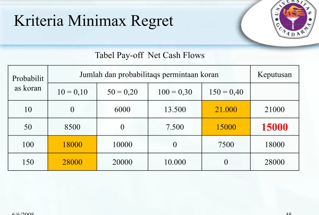
Kriteria Minimax Regret

• Menghitung kemungkinan regret untuk masing-masing alternatif di bawah masing-masing state nature.

• Mengidentifikasi kemungkinan regret maksimum untuk masing-masing alternatif.as g as g a te at .

• Memilih alternatif dengan regret maksimum yang terendah. Perhitungan tabel regret

P ff P ff l d Outcome regret baru = Payoff maksimum dari suatu kolom

Payoff lama pada baris dan kolom

masing-masing

(46)

-Kriteria Minimax Regret

Kriteria Minimax Regret

Probabilit as koran

as koran _{10 = 0,10} _{50 = 0,20} _{100 = 0,30} _{150 = 0,40}

10 0 6000 13.500 21.000

50 8500 0 7 500 15000

50 8500 0 7.500 15000

(47)

Kriteria Minimax Regret

Probabilit as koran

as koran _{10 = 0,10} _{50 = 0,20} _{100 = 0,30} _{150 = 0,40} 10 0 6000 13.500 21.000 1500 50 8500 0 7 500 15000 6500 50 8500 0 7.500 15000 -6500 100 18000 10000 0 7500 -16500 150 28000 20000 10 000 0 26500 150 28000 20000 10.000 0 -26500

(48)

Kriteria Minimax Regret

Probabilit as koran

10 = 0 10 50 = 0 20 100 = 0 30 150 = 0 40 y 10 0,10 50 0,20 100 0,30 150 0,40 10 0 6000 13.500 21.000 21000 50 8500 0 7 500 15000 15000 50 8500 0 7.500 15000 15000 100 18000 10000 0 7500 18000

(49)

Expected Value of Perfect

Information

i i i dih d i l h k id k i Disini dihadapi masalah ketidak pastian.

Untuk itu perlu dicari informasi tambahan diasumsikan Untuk itu perlu dicari informasi tambahan , diasumsikan

diperoleh informasi tambahan tentang permintaan, maka akan diperoleh nilai expected value of perfect information (EVPI):

EVPI =

Expected return jika

diperoleh informasi - Expected return tanpa

informasi sempurna

(50)

Expected Value of Perfect

Information

EVPI =

{(0,10 x 1500) + (0,20 x 7500) + (0,30 x 15000) + (0,40 x 22500) – 8350}

=

15150 8350

=

15150 – 8350

=

6800 Æ

jumlah untuk memperoleh informasi

yang sempurna

EMV = {(0,10x18000) + (0,20x10000) + (0,40x7500)}

(51)

Keputusan dalam kondisi resiko dan

fungsi utilitas

d l d h d

Amad pasang lotre Rp. 500 dengan harapan menang dapat Rp 500 juta. Probabilitas kalah dalam lotre adalah 99,99% dan probabilitas menang undian adalah 0,01%, maka expected

p g , , p

return-nya adalah:

= -500 (99,99%) + 500.000.000 (0,01%) = -499,95 + 50.000

(52)

Incorporating Risk Attitudes: Certain

Equivalent

I i i l l h $1000 d f i Initial wealth $1000, and you face two options:

(a) Keep your initial wealth and do nothing;

(b) Invest: receive $10,000 if succeed; lose 1000 if fail. After assessing these two options, you find

yourself indifferent between two. Analysis:

(53)

Risk Attitudes

Scenario: A person has two choices a sure thing and a

Scenario: A person has two choices, a sure thing and a

risky option, and both yields the same

expected value.

• Risk averse: take the sure thing

• Risk neutral: indifferent between two choices

• Risk loving: take the risky option

(54)

(55)

Risk Premium: Preventive

Investment

Initial wealth = 40 which results in U(40) = 120. An preventive

investment can magically ensure no disease outbreak (not realistic).

(a) Without disease outbreak, U(70) = 140

(b) With disease outbreak, U(10) = 70

70

(c) 0.5U(70) + 0.5U(10) = 105 Questions:

Questions:

(a) Will invest on preventive activities?

(b) Risk premium? (b) Risk premium?

(56)

Risk Premium: Earthquake Insurance

h li i h i f lif i h h

Josh lives in the San Francisco Bay Are of California where the prob. of an earthquake is 10%. His utility function is U(w) = w0.5, where w is wealth. If Josh chooses not to buy insurance , y next year, his wealth is $ 500,000 without an earthquake, and $ 300,000 at the lose of his house with an earthquake. What’s his risk premium?

(57)

Utility Theory

• Sometimes the decision with the highest EMV is not the most desired or most preferred alternative.

• Consider the following payoff table, S f N State of Nature Decision 1 2 EMV A 150,000 -30,000 60,000 <--maximum B 70,000 40,000 55,000 Probability 0.5 0.5

Decision makers have different attitudes toward risk:Decision makers have different attitudes toward risk:

• Some might prefer decision alternative A, • Others would prefer decision alternative B.

Utilit Th i t i k f i th d i i ki

Utility Theory incorporates risk preferences in the decision making

(58)

Constructing Utility Functions

• Assign utility values of 0 to the worst payoff and 1 to the best. • For the previous example,

U(-$30,000) = 0 and U($150,000) = 1

• To find the utility associated with a $70,000 payoff identify the valueTo find the utility associated with a $70,000 payoff identify the value pp atat which the decision maker is indifferent between:

Alternative 1: Receive $70,000 with certainty.

Alternative 2: Receive $150 000 with probability p and lose $30 000 with Alternative 2: Receive $150,000 with probability p and lose $30,000 with

probability (1-p).

(59)

Constructing Utility Functions

• If we repeat this process with different values in Alternative 1, p p , the decision maker’s utility function emerges (e.g., if

U($40,000) = 0.65): Utility Utility 0.80 0.90 1.00 Utility 0.80 0.90 1.00 Utility 0.40 0.50 0.60 0.70 0.40 0.50 0.60 0.70 0 00 0.10 0.20 0.30 0 00 0.10 0.20 0.30 0.00 -30 -20 -10 0 10 20 30 40 50 60 70 80 90 100 110 120 130 140 150 Payoff (in $1,000s) 0.00 -30 -20 -10 0 10 20 30 40 50 60 70 80 90 100 110 120 130 140 150 Payoff (in $1,000s)

(60)

Comments

• Certainty Equivalent - the amount that is equivalent in the

decision maker’s mind to a situation involving risk.

( $70 000 i l Al i 2 i h 0 8)

(e.g., $70,000 was equivalent to Alternative 2 with p = 0.8)

• Risk Premium - the EMV the decision maker is willing to

give up to avoid a risky decision

give up to avoid a risky decision.

(61)

Using Utilities to Make Decisions

• Replace monetary values in payoff tables with utilities.

Consider the utility table from the earlier example,Consider the utility table from the earlier example,

State of NatureExpected Decision 1 2 Utility A 1 0 0.500 B 0.8 0.65 0.725 <--maximum P b bilit 0 5 0 5 Probability 0.5 0.5

Decision B provides the greatest utility even though it the

payoff table indicated it had a smaller EMV. payoff table indicated it had a smaller EMV.

(62)

The Exponential Utility Function

• The exponential utility function is often used to model classic riskThe exponential utility function is often used to model classic risk averse behavior:

_U(

_x

₎

₌

₁

_-

_e

-x/R

(63)

I

ti

Utiliti i T

Pl

Incorporating Utilities in TreePlan

• TreePlan will automatically convert monetary values to utilities using • TreePlan will automatically convert monetary values to utilities using

the exponential utility function.

• We must first determine a value for the risk tolerance parameter R.

R i i l h i l f Y f hi h h d i i

• R is equivalent to the maximum value of Y for which the decision maker is willing to accept the following gamble:

Win $Y with probability 0.5,p y Lose $Y/2 with probability 0.5.

• Note that R must be expressed in the same units as the payoffs! • In Excel insert R in a cell named RT (Note: RT must be outside the

• In Excel, insert R in a cell named RT. (Note: RT must be outside the rectangular range containing the decision tree!)

• On TreePlan’s ‘Options’ dialog box select,

‘Use Exponential Utility Function’ ‘Use Exponential Utility Function’

(64)

Minimizing Variance or Standard

Deviation

• The payoffs of all events = X₁, X₂, X₃, . . . . , X_n

• The probability of each event = p₁, p₂, p₃, . . . . ., p_n • Expected value of x = • Variance =

∑

= = + + + + = n 1 i i i n n 3 3 2 2 1 1 X x .p x .p x .p ... x .p x .p EV • Variance =

(65)

Risk Measurement Absolute Risk:

Overall dispersion of possible payoffs Measurement: variance Overall dispersion of possible payoffs Measurement: variance, standard deviation

The smaller variance or standard deviation, the lower the absolute risk.

Relative Risk

Variation in possible returns compared with the expected payoff p p p p y amount

Measurement: coefficient of Variation (CV), The lower the CV, the lower the relative risk EV

(66)

Principles of Baye’s Strategy

Principles of Baye s Strategy

j b d k l i h d

• A project must not be undertaken unless it has an expected value that shows a profit

• The optimum decision would be the alternative that gives theThe optimum decision would be the alternative that gives the highest expected value of profit

(67)

Probabilities and Expected Values

Baye’s Strategy

• If probabilities are assigned to outcomes

– Decision is based on: The expected value which is the weighted average of these outcomes

(68)

Expected Value

d l

• Expected value EV

• x : denotes value of each possible outcome

(69)

Ill

i

Forecast of profit of a project

Illustration :

Forecast of profit of a project Profit / (Loss) $k p

EV = - 0.1 * 800 - 0.3 * 200 + 0.4 * 400

+ 0.2 * 500 = +120 k

Applying Baye’s Strategy

Decision: Go ahead with the project although a 0.4 probability of making a loss exists

(70)

Example:

3 ll l i i A B C 3 mutually exclusive options, A, B, C

Each option has three possible outcomes:

I with P(I) = 0.1 ; II with P(II) = 0.7 ; III with P(III) = 0.2 Conditional Profits ($k)

Profit ($k)

I II III

(71)

Solution

EV of Options

Solution

EV of Options A: 0.1 * 20 + 0.7 * 60 + 0.2 * 80 = $ 60 k B: 0.1 * ( - 30 ) + 0.7 * 80 + 0.2 * 120 = $ 77 k C: 0.1 * 10 + 0.7 * 40 + 0.2 * 150 = $ 59 k Option B is preferred

(72)

M

f Di

i

• Variance (σ 2)

Measures of Dispersion

( )

– A measure of the spread of probability distribution

• Consider a random variable x

Let its expected value E(x) be µ

– Let its expected value E(x) be µ

(73)

Let x be a random discrete variable taking values xn and probability pn

σ2 ₌_{E(x - µ)}2

= p₁ (x₁ - µ)2 _{+ p}

2 (x2 - µ)2 +.. + pn (xn- µ)2 Standard deviation σ = √E(x −µ)2

Coefficient of variation (COV) = µ / σ

COV - a measure of the risk involved COV a measure of the risk involved

(74)

Example

Land development projects in two districtsp p j

(75)

Solution

Expected value of net annual income Solution p E(x) = µ = Σ xi pi District A District A µ = 0.15 * 600 + 0.20 * 700 + 0.30 * 800 + 0.20 * 900 + 0.15 * 1000 = 800.0 District B µ = 0.15 * 770 + 0.20 * 790 + 0.30 * 800 + 0.20 * 810 + 0.15 * 830 = 800.0 • Expected values are the same

(76)

Measures of Risk

bl f i i k

• An acceptable way of measuring risk

– Examine the probability distribution of the outcomes (annual net incomes)

(77)

(78)

(79)

(80)

Decision Trees

A di i i f ll h l i l ibili i f

• A diagrammatic representation of all the logical possibilities of a sequence of events

• Each event can occur in a finite numberof ways

• Displays the full range of alternative actions that can be taken

• Each decision by its nature limits the scope of later decisions

• An estimated value for each possible outcome is required p q

• The estimated values multiplied by their probabilities are "rolled back" to the start of the tree

(81)

Illustration

h l d i i d b h d

The Flood Protection Agency is concerned about the damages that could be caused by a hurricane, if it strikes. It is aware that damages can be considerably reduced if a breakwater is built. g y Suppose the following estimates are made:

(82)

Estimates

P b bili f h i i i d i h l i h i

• Probability of a hurricane occurring in ayear during the planning horizon: p

• Damages if a hurricane strikes without the protection of a breakwater: D

• Damages if a hurricane strikes with the protection of a breakwater:

q * D (q<1)

• Equivalent annual cost (during the planning horizon) of building a breakwater: C

(83)

(84)

Creating the Decision Tree Model

Procedure

• Current Situation (Location 1) is a decisionmaking situation with two alternatives:

– No protectionNo protection

– Build breakwater at cost C • Location 1 is a Decision Node

D b h h l i

• Draw branches to represent the alternatives – A future situation (Location 2)

(85)

Creating the Decision Tree Model

Af h d i i

• After the decision

Location 2 or 3 becomes "current" situation

• Location 2 and 3 are Chance Nodes

• At chance nodesAt chance nodes

• No decision is made

• One of many possible outcomes will occur

Th ibl t d b h ti f h f th

• The possible outcomes drawn as branches emanating from each of the chance nodes

(86)

Creating the Decision Tree Model

If h f h i i

• If there are no further situations

• The cost consequence for each outcome is indicated at the end of the branch

(87)

(88)

W k h ll l b h i COST d • W is taken as the smaller value because the consequence is COST and a

smaller cost would lead to a larger profit (Bayes’ Strategy)

(89)

Example: Computer cards problem

P i 20 d f i

• Past experience: 20 percent defective

• Two inspectors X and Y to check cards and mark • Ok if Good

• Not Ok if Bad

• Probability of wrong classification = 0.1

(90)

(91)

P (C l l ifi d) 0 648 0 162 0 018 0 018 0 846 P (Correctly classified) = 0.648 + 0.162 + 0.018 + 0.018 = 0.846 Defective cards reaching customers

(92)

(93)

(94)

l f f i Value of Information

• Probabilities assigned to outcomes depend on the information available

available

• Accuracy can be improved with better information • How much is such information worth?

(95)

id l i i Consider example on Investment Decision • If there is "Market" for the product

• Best option : High Investment • Best option : High Investment

: Profit $100 m

• If there is "No Market" for the product If there is No Market for the product • High Investment:Loss $ 60 m

• Low Investment: Loss $ 4 m

(96)

(97)

• EV with perfect information : $ 80 m

• EV without information : $ 68 m

• Value of perfect information = $ 80 m $ 68 m = $12 m

(98)

Value of Imperfect Information

f i f i i h d b

• Perfect information is hard to come by.

• Continued from the previous example, decision-maker D hires Management Consultant firm MC to carry out market

Management Consultant firm, MC, to carry out market survey.

• Accuracy of MC’s prediction: – 85% accurate

(99)

(100)

i h i f i f i $

EV with imperfect information : $ 62.4 m EV without information : $ 68 m

Value of imperfect information = $ 62 4 m $ 68 m = $ 5 6 m Value of imperfect information = $ 62.4 m - $ 68 m = - $ 5.6 m

(101)

KEPUTUSAN DALAM SUASANA RISK

( DENGAN PROBABILITA )

Tahap-tahap:

1. Diawali dengan mengidentifikasikan

bermacam-macam tindakan yang tersedia dan layak

macam tindakan yang tersedia dan layak

2. Peristiwa-peristiwa yang mungkin dan probabilitas

terjadinya harus dapat diduga

j

y

p

g

3. Pay off untuk suatu tindakan dan peristiwa tertentu

ditentukan

(102)

Probabilitas dan Teori Keputusan

BAGIAN Probabilitas dan Teori Keputusan

Konsep-konsep Dasar Probabilitas

Distribusi Probabilitas

Pengertian dan Elemen-Elemen Keputusan

Pengambilan Keputusan dalam

Distribusi Probabilitas Diskret

g p

Kondisi Risiko (Risk)

(103)

Teknik yang digunakan

:

a. Expected Value (Nilai Ekspektasi)

Teknik yang digunakan

:

b. Expected Opportunity Loss ( EOL )

Untuk meminimumkan kerugian yang disebabkan karena pemilihan

alternatif keputusan tertentu. Keputusan yang direkomendasikan criteria p p y g expected value dan expected opportunity loss adalah sama, dan ini bukan suatu kebetulan karena kedua metode ini selalu memberikan hasil yang

sama, sehingga cukup salah satu yang dipakai, tergantung tujuannya. Hanya criteria ini sangat tergantung pada perkiraan probabilita yang akurat.

c. Expected Value of Perfect Information (EVPI)

Merupakan perluasan dari criteria EV dan EOL, atau dengan kata lain p p g

informasi yang didapat pengambil keputusan dapat mengubah suasana risk menjadi certainty (membeli tambahan informasi untuk membantu pembuat keputusan). EVPI sama dengan EOL minimum (terbaik), karena EOL

(104)

Teknik yang digunakan

:

d Expected Value of Sample Information (EVSI)

Teknik yang digunakan

:

d. Expected Value of Sample Information (EVSI)

Merupakan harapan yang diinginkan dengan tambahan informasi untuk dapat mengubah /memperbaiki keputusan, dengan menggunakan teori Bayes.

e. Kriteria Utility dalam suasana risk EV max / EOL min tidak selalu digunakany g

sebagai pedoman dalam mengambil keputusan, hal ini terjadi karena:

1. Orang lebih memilih terhindar dari musibah potensial daripada mewujudkan

keuntungan dalam jangka panjang

2. Orang lebih memilih mendapatkan/memperoleh rejeki nomplok daripada

(105)

PERSOALAN INVENTORI SEDERHANA

DALAM KEADAAN ADA RISIKO

Kriteria nilai harapan (expected value) yang telah digunakan di Kriteria nilai harapan (expected value) yang telah digunakan di atas juga diterapkan untuk memecahkan persoalan inventori

(106)

GAME THEORY

(Pengambilan Keputusan Dalam Suasana Konflik)

Adalah memusatkan analisis keputusan dalam suasana konflik Adalah memusatkan analisis keputusan dalam suasana konflik dimana pengambil keputusan menghadapi berbagai peristiwa yang aktif untuk bersaing dengan pengambil keputusan lainnya, yang rasional, tanggap dan bertujuan memenangkan persaingan/kompetisi.

(107)

Pengelompokan Game Theory:

1. berdasarkan Jumlah Pemain:

Pengelompokan Game Theory:

a. Two-persons games b. N-persons games

2. Berdasarkan Jumlah Pay off: 2. Berdasarkan Jumlah Pay off:

a. Zero and constan sum games

b. Non zero and non constan sum games 3 B d k St t i di ilih

3. Berdasarkan Strategi yang dipilih: a. Cooperative games

b. Non cooperative games 4. Fokus pembahasan:

5. Two-persons, zero and constan sum games 6. Asumsi dalam game theory:

6. Asumsi dalam game theory:

a. Setiap pemain mengetahui dengan tepat pay off setiap kemungkinan kombinasi strategi yang tersedia.

(108)

Caranya:

1. Prinsip Maximin dan Minimax

Caranya:

1. Prinsip Maximin dan Minimax

Karena nilai maximin = minimax, maka disebut matriks games mempunyai saddle point atau value of games senilai saddle point tersebut Bila setiap pemain tidak berkeinginan merubah satu strategi tersebut. Bila setiap pemain tidak berkeinginan merubah satu strategi yang telah dipilih, maka games itu merupakan “pure strategy”

2. Peranan Dominasi

Suatu strategi dikatakan mendominasi apabila selalu menghasilkan pay off lebih tinggi dibandingkan dengan strategi yang lain. Strategi yang

(109)

Caranya:

i d

3. Mixed Strategy

Menentukan probabilitas (kemungkinan) strategi yang ada yang digunakan dalam pertarunngan (kalau tidak ada “pure yang digunakan dalam pertarunngan (kalau tidak ada pure strategy/tidak ada saddle point”)

Caranya:

a. Pendekatan EV / EG (expected Gain) b. Pendekatan EOL

M k il i i

(110)

ANALISIS MARKOV

Analisis ini tidak memberikan keputusan rekomendasi, tetapi Analisis ini tidak memberikan keputusan rekomendasi, tetapi memberikan informasi probabilita situasi keputusan yang dapat

membantu pengambil keputusan untuk membuat keputusannya, dengan kata lain bahwa analisis markov bukan merupakan teknik optimasi, tetapi kata lain bahwa analisis markov bukan merupakan teknik optimasi, tetapi merupakan teknik deskriptif yang menghasilkan informasi probabilita. Asumsi:

1 b bili b i b j l h d 0

1. Probabilita baris berjumlah sama dengan 0