Mathematics and Informatics ICTAMI 2005 - Alba Iulia, Romania
GENETIC METHODS USED IN ARTIFICIAL NEURAL NETWORKS DESIGN
Ioan Ilean˘a, Corina Rotar, Ioana Maria Ilean˘a
Abstract. In the Artificial Intelligence field, two areas have attracted a lot of attention in the past years: Artificial Neural Networks (ANN’s) and Genetic Algorithms (GA). The artificial neural networks, by their capacity to learn non-linear relationships between an input and an output space have a lot of applications: modeling and controlling dynamic processes and systems, signal processing, pattern recognition, forecast etc. There are many types of ANN, the most used being the feed forward neural networks and the recurrent neural networks. The design and the training of such ANN’s may be optimized by using genetic techniques. In this paper we present several results related to: feature selection in pattern recognition, optimization of feed-forward neural networks structure and the determinations of the spurious attractors of an associative memory by using evolutionary algorithms.
Key words: genetic algorithms, feature selection, feed forward neural net-work, autoassociative memory
1. Genetic algorithms and their applications
Genetic algorithms proved to be adequate tools for solving different kind of problems, especially optimization problems. They are preferred in many situ-ations, especially when a good approximation could satisfy our needs. More-over, genetic algorithms do not require supplementary conditions regarding optimized function, as the traditional methods do, and they are comprehensi-ble and easy to implement.
Each element of the population is called chromosome and codifies a point from the search space. The search is guided by a fitness function meant to evaluate the quality of each individual. The efficiency of a genetic algorithm is connected to the ability of defining a ”good” fitness function. For example, in real function optimization problems, the fitness function could be the function to be optimized.
The paper summarizes several applications of the Genetic Algorithms in ANN’s area. Two of the following problems are multicriterial optimization problems and the last presented one represents a multimodal optimization problem. We apply genetic techniques for each case and present the results in the next paragraphs.
In the second section of the paper the feature selection problem is solved by using two different evolutionary multicriterial techniques: Weight Sum Ap-proach and an aggregation technique. The mentioned algorithms are detailed presented in the paragraph 1.2.
In the third section of the paper the optimization of feed forward neural networks structure problem is presented. We also detected this problem as a multicriterial optimization problem and we applied the specific evolutionary methods described in paragraph 1.2: Weight Sum Approach (an aggregation technique) and recently developed multicriterial method, MENDA.
The fourth section is dedicated to the Associative Neural Memory’s At-tractors Determination by using genetic algorithms. This problem represents a multimodal optimization problem and we applied in this case a well-known niching method: fitness sharing technique, described in paragraph 1.1.
1.1. Evolutionary Algorithms and Multimodal Optimization Standard genetic algorithm has a difficulty regarding multimodal optimiza-tion problems. The main weakness of the standard genetic algorithm consists in its premature convergence toward a single optimum of the specified func-tion. Due to this, a supplementary technique for diversity preservation must be used. We choose to make use of a niching method, respectively, fitness sharing [7], to find simultaneously more than one optimum. The idea of this technique is to establish subpopulations in the population. Each subpopu-lation corresponds to an optimum and finally, the genetic algorithm returns multiple solutions of the problem.
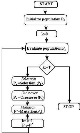
Figure 1: Standard Genetic Algorithm
For establishing the degree of sharing between each pair of individuals, a dis-tance d is taken into consideration. The sharing function is defined as an application:
s :R −→[0,1] , which verifies the next assertions: 1. s is decreasing
2. s(0) = 1 3. lim
d−→∞
s(d) = 0
The statements from above could be explained as follows: if the distance between individuals is great, the degree of sharing is small, and, if the indi-viduals are close, the degree of sharing became great. The fitness function is modified as follows:
f∗ (xi) =
f(xi)
mi
mi = n X
j=1
s(d(xi, xj)) (2)
The modified fitness function is called shared fitness function.
The genetic algorithm for detecting spurious attractors is described in sec-tion 4. First, each individual (chromosome) of the populasec-tion codifies a pos-sible solution. A potential solution represents a pattern that might be memo-rized by the neural net.
A possible pattern is a black and white image of n×n pixels represented by a n-by-n matrix of 1 and –1. We applied the genetic algorithm for 2-by-2, 3-by-3 and 4-by-4 matrices. The possible lengths of the chromosomes are 4, 9 or 16.
An individual is a binary string of constant length. The binary alphabet is {−1,1}. The population evolves by applying the genetic operators: binary tournament selection, one-position uniform mutation and uniform crossover.
For measuring the distance between two individuals, a = (a1, a2, . . . am)
and b = (b1, b2, . . . bm), the number of different corresponded genes of those
individuals is counted:
d=
m X
i=1
wi, and wi =
1 if ai 6=bi
0 otherwise (3)
The sharing function is build:
s(d) =
(
1− 1
ad if d < a
0if d≥a (4)
where a represents an extra parameter of the genetic algorithm. The value of the parametera represents the maximum number of different corresponded genes of two individuals considered as belonging to the same niche. The main weakness of the method relies on defining a “good” value for the parametera.
These objectives are usually in conflict. So, the optimization term is used in the sense of determination of a solution that gives acceptable values to all objectives.
Formally, the multi-criteria optimization problems are define in the follow manner: find the next vector:
¯ x∗ = x∗ 1 ... x∗ n (5)
Which will satisfy the constraints:
gi(¯x)≥0, i= 1, ..., m (6)
hi(¯x)≥0, i= 1, ..., p (7)
And optimize the vector function:
¯ f(¯x) =
f1(¯x) ... fk(¯x)
(8)
Where ¯x represents the vector of decision variables.
We note withF the set of the values, which satisfies (5) and (6). This setF symbolizes the feasible region from the search space. Thus, we are interested to determine from the set F, all particular values x∗
1, ...x ∗
n, which produce
optimum values of the objective functions.
Each ¯x point from the feasible region F defines a feasible solution. The main problem is that the concept of optimum is not too clearly defined in the context of multiple objectives. We rarely find the next situation:
fi(¯x
∗
)≤fi(¯x), f or every x¯∈F, i= 1,2, ..., k (9)
where ¯x∗
is the desired solution.
Actually, the situation described earlier is exceptional: we seldom locate a common point ¯x∗
for which all fi(¯x) have a minimum. Because of this
Pareto Optimum
Vilfredo Pareto firstly introduced and formulated the most popular concept of optimality. The vectorx∗
∈F of decision variable isPareto optimal if there isn’t another vector x∈F such as:
fi(x)≤fi(x
∗
) f or every i= 1,2, ..., k (10)
It exists j = 1,2, ..., k, such that fj(x)< fj(x
∗
) (11)
This concept of optimality guides us unfortunately not to a single solution but rather to a set of solutions. Eachx∗
vector that corresponds to a solution from the Pareto set is called non-dominated. The region fromF that is formed by the non-dominated solutions represents the Pareto front.
Evolutionary approach
For solving the above problem we used two evolutionary approaches: one approach that doesn’t use the concept of Pareto dominance when evaluating candidate solutions (non Pareto method) - weights method - and one Pareto approach recently developed inspired by endocrine system.
Non-Pareto method (Weights method)
The technique of combining all the objective functions in one function is denoted the function aggregation method and the most popular such method is the weights method.
In this method we add to every criterion fi a positive sub unity value wi
denoted weight. The multicriteria problem becomes a unicriteria optimization problem.
If we want to find the minimum, the problem can be stated as follows:
min
k X
i=1
wifi(¯x) (12)
0≤wi ≤1, (13)
Usually
k X
i=1
The main advantages of this method consists in the facts that the aggrega-tion technique is simple to implement and easy to understand. One drawback of this method is the determination of the weights if one don’ know many things about the problem to be solved. Another disadvantage of the aggrega-tion techniques against the Pareto based techniques, is given by the fact that the second class of methods (Pareto-based) provide an entire set of solutions (Pareto front), from which we can further choose an appropriate one for our purpose.
Pareto method
We have applied a recently developed method inspired by the natural en-docrine system .
The main characteristics of this method are:
1. It maintains two populations: one active population of individuals (hor-mones) H, and one passive population of non-dominant solutions T. The members of passive T population act like an elite collection having the func-tion of guiding the active populafunc-tion toward Pareto front and keeping them well distributed in search space.
2. The passiveT population doesn’t suffer any modifications at individuals’ level through variation operators like recombining or mutation. In the end the T will contain a previously established number of non-dominating vectors supplying a good approximation of thePareto front.
3. At each T generation the members of the Ht active population are
divided instclasses, wherestrepresents the number of tropes from the current T population. Each hormone class is supervised by a correspondent trope. The point is that eachhhormone fromHtis controlled by the nearestai trope from
At .
4. Two individuals’ evaluation functions are defined. The value of the first one for an individual represents the number of individuals of the current population that are dominated by it. The value of the second function for an individual represents the agglomerate degree from the class corresponding to that particular individual.
A more detailed presentation of the MENDA technique is presented in the reference 22.
2. Genetic algorithms in feature selection
In many areas like pattern recognition, machine learning, data mining, one use features vectors of great dimensionality as reality representations. The great number of vector components increases the running time and the cost of the process. Moreover some features in this vector may be irrelevant, redun-dant or noisy. The applications in these fields often require a feature selection in order to reduce input space dimension, and therefore obtain a reasonable execution time. These are the reasons for the reduction of feature vector com-ponents number by the feature selection/extraction process that intends to obtain a set of features having the following characteristics: discrimination, independence, small numbers and reliability.
There are several “traditional” methods for operating this reduction (e.g. Karhunen-Loeve); however, in this section we attempt to implement feature selection using genetic algorithms. We use neural networks for pattern recog-nition and the theoretical assumptions will be verified when performing 2D image recognition. The genetic algorithms perform the reduction of the input vectors, retaining a smaller number of components, which are significant for and concentrate the essential characteristics of the classes to be recognized.
Actually there are two general approaches: features transformationand feature selection[18]. Feature Transformation (Feature Extraction) is a pre-processing technique that transforms the original features of a data set to a set of new features, smaller, more compact, while retaining as much information as possible.
Feature Selection is concerned with finding a subset of features from the original features so that the feature space is optimally reduced according to one or more criteria, rather than producing an entirely new set of dimensions for the data. In this paper we are dealing with the second approach, feature selection in the field of pattern recognition (classification), and we will do this selection by means of genetic algorithms.
2. 1. Approaches in features selection
of training samples. As a consequence, the selection of the best discriminative features plays an important role when constructing classifiers. However, this is a difficult task especially when dealing with a great number of features. In the above context, feature selection presents a multi-criterion optimization process, and the set of optimal features can be different for different hypothesis spaces [2].
The problem of feature selection may be stated as follows: choose a min-imum subset of M features from the original set of N features (M < N), so that the feature space is optimally reduced according to a certain evaluation criterion. In the case ofN features, the total number of features combinations is 2N. Finding the best feature subset is usually intractable and many
[image:9.612.158.434.335.431.2]prob-lem related to feature selection have been shown to beNP-hard [14]. Feature selection is, in general a search process, consisting of four basic steps: sub-set generation, subsub-set evaluation, stopping criterion, and result validation, as illustrated in Figure 2.
Figure 2: General Procedures of Feature Selection. Source: [14]
An important aspect is how to measure the goodness of a feature subset. Based on their dependence on the learning algorithm applied on the selected feature subset, evaluation criteria can be broadly categorized into two groups: filter models and wrapper models.
In filter models an independent criterion tries to evaluate the goodness of a feature or feature subset without the involvement of a learning algorithm in this process. Some of the independent criteria are distance measure, infor-mation measure, dependency measure, consistency measure.
Recently, hybrid models are proposed to combine the advantages of both filter models andwrapper models in the context of handling exponentially high dimensionality [14].
Other criterion of classification of features selection approaches is the avail-ability of class information in data: there are supervised feature selection approaches and unsupervised feature selection approaches. There are many algorithms for feature selection and several taxonomies.
2.2. Our Approach
In our present work we will use multi-criteria optimization function, at-tempting to decrease the number of features used to classify images and in the same time to increase the discriminate power of retained features. Genetic algorithm (GA) offers a particularly attractive approach to solve this kind of problems since they are generally quite effective in rapid global search of large, non-linear, and poorly understood spaces. We will use a multi-objective GA to perform feature selection, as described in next section. Our approach be-longs to the filter methods with nondeterministic generation of subsets and a distance evaluation criterion.
Work methodology. Description of the applied algorithm
We used the presented GA in order to reduce the number of features in an images classification context. The classifier is of ANN type and is designed to recognize the handwritten digits 0. . .9. The training set is represented by 16×16 pixels black/white images (prototypes) of the digits from Figure 3.
Figure 3: Digit images used to train the classifier
In this situation each pixel of the image represents one feature and we try to see what the minimum number of pixels is which permit to discriminate between the 10 training images. The objective of the feature selection is: find-ing the minimum number of pixels that yields the maximum mean Hammfind-ing distance between training prototypes.
prototype. Concrete, we used white/black images of 16x16 pixels, resulting a vector of 256 elements 0 (white) or 1(black).
In the implemented genetic algorithm we have considered that each indi-vidual (chromosome) of population represents a vector of n elements (where n represents the number of pixels of the pattern, e.g. 256), the value of each element being 1 or 0 with the signification:
• 1 , if the corresponding feature (pixel) is selected
• 0, in contrary.
We define the length of a chromosome by the number of elements equal with 1 in the framework of the vector. The performance of a chromosome is much better as the length is shorter, the number of selected features is smaller, respectively. This way results the first criterion implied into the searching and optimization process.
Practically, each chromosome represents an extracting mask of a vector of features from the initial vectors. A chromosome is as much better as much it is capable to extract features that produce un-like extracted vectors. In order to measure the level of similarity between any two vectors of elements 0 and 1 we have considered the Hamming distance. For each chromosome/individual of population there will be extracted 10 vectors of features of the initial vectors. More these extracted vectors are less similar more the quality/performance (fitness) of the chromosome is better.
The second criterion of the problem is proportional with the inverse of the average of the Hamming distances between any two vectors produced after the features’ extraction from the initial vectors. This criterion has to be minimized as well.
2. 3. Practical Results
We have applied two methods of aggregation of objectives: 1. First method is the weight sum approach.
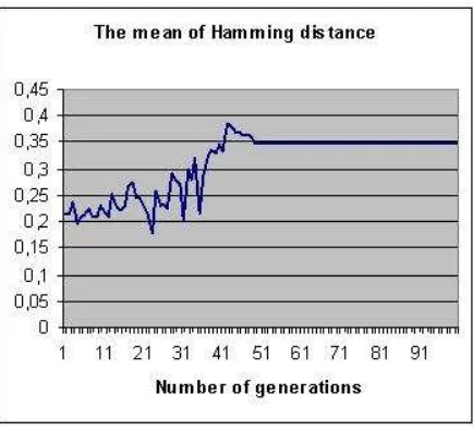
As regards the selection method we have chosen the proportional selection on the fitness of chromosomes. The genetic operator used is the recombination with a single point of cut. We used 100 individuals’ populations and the 100 generations. The results are displayed in figures 4, 5, 6, 7 for the two approaches used.
In the first approach, the length of features vector decreases continuous and after 50 generations stabilizes at a value of 8 features. In the same time one can see an increase of mean Hamming distance between vectors, which stabilizes at a value of 0.35.
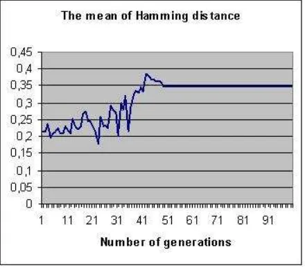
[image:12.612.187.406.274.453.2]In the second approach, illustrated by figures 6 and 7, the vector length stabilizes at 13 features and the mean of Hamming distance is 0.42.
Figure 5: Mean of Hamming distance between vectors
[image:13.612.188.405.351.549.2]Figure 7: Mean of Hamming distance between vectors
3. The optimization of feed forward neural networks structure using genetic algorithms
Artificial neural networks (ANNs) are an interesting approach in solving some difficult problems like pattern recognition, system simulation, process forecast etc. The artificial neural networks have the specific feature of “storing” the knowledge in the synaptic weights of the processing elements (artificial neurons). There is a great number of ANN types and algorithms allowing the design of neural networks and the computing of weight values.
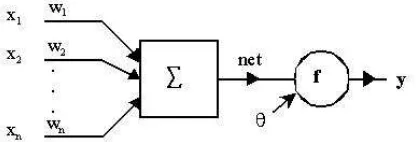
Figure 8: The model of artificial neuron used
In this figure x1, x2, ...xn are neuron’s inputs, w1, w2, ...wn are
intercon-nection weights, Θ is neuron’s threshold, f() is activation function and y is neuron’s output. We shall denote x = [x1, x2, ..., xn]T input vector, w =
[w1, w2, ..., wn]T synaptic connections vector, Θ thresholds vector,
net=X
i
wixi =wTx (15)
The output of the neuron may be written:
y=f(net−Θ) =f(wTx−Θ) (16) In practical applications, the neural networks are organized in several layers as shown in Figure 9.
3.1. Design Approaches for Feed-Forward Neural Networks Implementing a RNA application implies three steps [4]:
• Choice of network model;
• Correct dimensioning of the network;
• The training of the network using existing data (synaptic weights syn-thesis).
This paper is dealing with feed-forward neural network so we concentrate on steps 2 and 3.
Network dimension must satisfy at least two criteria:
• The network must be able to learn the input data ;
Figure 9: Multilayer feed-forward neural network
The accomplishment degree of these requirements depends on the network complexity and the training data set and training mode. Figure 10 shows the dependence of network performance in function of the complexity and Figure 11 shows the same dependence of the training mode.
Figure 10: Performance’s dependence of network complexity. Source: [4], p. 74
[image:16.612.220.363.406.519.2]Figure 11: Performance’s dependence of the training mode. Source: [17], p. 40.
to an increased training speed and to lower implementation cost.
The designing of a feed-forward structure that would lead to the minimizing of the generalization error, of the learning time and of the network dimension implies the establishment of the layer number, neuron number in each layer and interconnections between neurons. At the time being, there are no formal methods for optimal choice of the neural network’s dimensions.
The choice of the number of layers is made knowing that a two layer network (one hidden layer) is able to approximate most of the non linear functions demanded by practice and that a three layer network (two hidden layers) can approximate any non linear function. Therefore it would result that a three layer network would be sufficient for any problem. In reality the use of a large number of hidden layers can be useful if the number of neurons on each layer is too big in the three layer approach. Concerning the dimension of each neuron layer the situation is as follows:
• Input and output layers are imposed by the problem to be solved;
Hidden layer dimensioning methods Type of method
Empirical methods Direct
Methods based on statistic criteria Indirect
Constructive Direct
Ontogenic methods Destructive Direct
Mixed Direct
Based on Genetic Algorithms Direct
Most methods use a constructive approach (one starts with a small number of neurons and increases it for better performances) or a destructive approach (one starts with a large number of neurons and drops the neurons with low activity).
As a general conclusion, there are a multitude of methods for feed-forward neural networks designing, each fulfilling in a certain degree the optimization requests upper presented.
3.3. The Proposed Optimization Approach
As we have previously seen, optimal designing of feed forward neural net-works is a complex problem and three criterions must be satisfied:
• The network must have the capacity of learning
• The network must have the capacity of generalization
• The network must have the minimum number of neurons.
Next we shall present one method of optimizing the network’s structure, by the use of Evolutionary Algorithms (EA). Evolutionary algorithms (par-ticularly, Genetic Algorithms) proved their efficiency in solving optimization problems and, moreover, many evolutionary techniques have been developed for determining multiple optima of a specific function.
According to the evolutionary metaphor, a genetic algorithm starts with a population (collection) of individuals, which evolves toward optimum solutions through the genetic operators (selection, crossover, mutation), inspired by biological processes [3].
real function optimization problems, the fitness function could be the function to be optimized. The standard genetic algorithm is illustrated in the Figure 12. The optimization of feed-forward neural networks structure represents a typical multicriterial optimization problem.
3.4. Experimental Results
We have applied the optimization method presented for a feed-forward neu-ral network synthesized to approximate the function illustrated in Figure 12. The non linear function approximated by the network. The train-ing and testtrain-ing data were different; even more the data used for testtrain-ing were outside training set.
[image:19.612.160.435.373.519.2]The chromosomes will codify the network dimension (number of layers, number of neurons on layer) and the fitness function will integrate the training error (after a number of 100 epochs), the testing error (as a measure of the generalization capacity) and the entire number of neurons of the network. To simplify we considered only two or three layers networks. The maximum number of neurons on each layer is 10. There is one output neuron. The obtained results are shown in tables 2, 3.
Figure 12: The non linear function approximated by the network
Weights method
Population dimension 20 Number of generations 100
Criteria F1 - training error, F2 - test error, F3 - inverse of neuron number
W1 1
[image:20.612.118.462.85.323.2]W2 1
Table 3.
MENDA Technique Population dimension 20
Number of generations 100
Criteria F1 – training error, F2 – test error
Solutions: (2,8)
[image:20.612.191.399.382.552.2]The structure obtained by the use of the optimizing algorithm was tested in Matlab and the results are shown in figures 13 and 14.
Figure 14: Output of the 1:4:1 network (+) compared with desired output (line)
4. Associative neural memory’s attractors determination by using genetic algorithms
One special type of ANN is the recurrent neural networks used as associa-tive memories with applications in pattern recognition. Such a memory can store a number of patterns (prototypes) and when one unknown pattern is presented at memory’s input, it recalls the appropriate prototype. The prob-lem is that, in the synthesis of the memory, are stored not only the desired prototypes but also some “spurious” patterns that manifest itself like memory attractors, modifying the dynamics of the network. These fixed points produce also a reduction of prototypes attraction basins and the designer’s interest is to reduce their number. Depending of the method of synthesis of the memory, a variable number of such unwanted fixed points can appear.
4.1. The Artificial Neural Network Model
In this section we’ll briefly introduce the main theoretical elements concern-ing associative memories and recurrent neural networks [12], elements that will be used in order to build an associative memory for patterns recognition.
We’ll call pattern a multidimensional vector with real components. An associative memory is a system that accomplishes the association of p pattern pairsξµ∈Rn, ςµ∈Rm,(µ= 1,2, ..., p) so that when the system is given a new
d(x, ξi) = min f d(x, ξ
j) (17)
the system responds with ςi; in (1) d(a, b) is the distance between patterns a
and b.
The pairs (ξi, ςi),(i = 1,2, ...p) are called prototypes and the association
accomplished by the memory can be defined as a transformation Φ :Rn×Rm
so thatςi = Φ(ξi). The space Ω⊂Rnof input vectorsxis named configuration
space and the vectors ξi, (i= 1,2, ..., p) are called attractors or stable points.
Around each attractor, there is a basin of attraction Bi such that x ∈ Bi,
the dynamics of the network will lead to the stabilization of (ξi, ςi) pair. For
autoasociative memories ςi =ξi.
[image:22.612.133.462.348.478.2]In this section we will use for graphic pattern recognition a neural network whose model [12] is presented below. Let’s consider the single-layer neural network built from totally connected neurons, whose states are given by xi ∈ {−1,1}, i= 1,2, ...n (Figure 15).
Figure 15: Single layer recurrent neural network We denote: W = [wij,: 1≤i, j ≤n] the weights matrix,
Θ = [Θ1, ...,Θn]T ∈Rn the thresholds vector,
x(t) = [x1(t), ...xn(t)]T ∈ {−1,1}n the network state vector.
Given a set ofn-dimensional prototype vectorsX = [ξ1, ξ2, ..., ξp],we
estab-lish the synaptic matrix W and the threshold vector Θ, so that the prototype vectors become stable points for the associative memory, that is:
ξ1 =sgn(W ξi−Θ), i= 1,2, ..., p (18)
where the sgn function is applied to each component of the argument.
We use the Lyapunov method to study the stability of the network, defining an energy function and showing that this function is decreasing for any network trajectory in the state space. In our case, we’ll consider the following energy function:
E(x) =−1
2x
TW x−xTΘ (19)
where x is the network state vector at timet.
From the evolution in states space point of view, a network can reach a stable point or can execute a limit cycle. At its turn, a stable point can be a global or a local energy minimum.
In paper we are dealing with the determinations of the energy minimum (attractors) of an associative memory in order to see which “legal” prototypes are and which spurious fixed points are. We use for this determination genetic algorithms like that used in multimode optimization. This work is impor-tant because determination of total number of attractors (memory’s energy minimums) can lead to optimization of memory’s synthesis using Hebb’s rule, projection rule or some other variants.
4.2. Methodology of Work
The genetic algorithm runs several times. The outcomes of each run are collected into a set U. The duplicates of the stored solutions are eliminated. Also, the real prototypes are removed. The final collection U contains the spurious attractors.
The results indicated below were found using the following parameters for the genetic algorithm:
• Population size = 100.
• Maximum number of generations = 100.
• lc (representing the length of the chromosomes) = 4(22),9(32),
• Parametera= 1 if lc = 4, a= 2 if lc = 9 and a= 6 if lc = 16, indicating
that each pair of individuals which differ in at most a genes belong to the same niche.
• The fitness function is given by energy functionE. The shared fitness is modified accordingly to formula (4).
4. 3. Results
We synthesized several autoassociative memories by using recurrent neural networks presented in 4.1.These memories store some simple graphical patterns as prototypes and for which of them we calculated the energy minima to detect all the memory attractors. For weight matrix synthesis we used Hebb’s rule or the projection rule and, for simplicity, we assumed value zero for thresholds of the neurons. We studied three types of autoassociative memories and the results are displayed below.
[image:24.612.109.484.381.469.2]Figure 16 show the patterns (prototypes) stored in first memory and re-spectively the attractors found by using the method described in section 1. The patterns are 2×2 pixels black and white images.
Figure 16: Results obtained for the first memory
One can see a great number of spurious attractors corresponding to energy local minima. This situation may be explained by the great number of proto-types attempted to be stored with a memory of only four neurons. Also one can remark the existence of pairs of attractors and their symmetric, due to the symmetry of synaptic matrix.
Figure 17: Results obtained for the second memory
[image:25.612.153.435.368.585.2]Finally we studied a memory which store 4×4 pixels images and in figure 5 the results are displayed.
In this case one can see that the spurious attractors are only the inverse of prototypes. This situation can be explained so: the number of neurons and the small number of prototypes assure the memory not to be saturated.
5. Conclusions and future works
A. Feature selection
In this work we used GA in order to optimize the images recognition by decreasing the features vector dimension and by increasing, in the same time the Hamming distance between vectors to be classified. As exemplars we used black and white images of the 0 to 9 digits.
The two approaches presented above shown that the GA are useful tools in reaching such goals, but with different tradeoffs. The weights method show yields a smaller feature vector but with the drawback of a smaller Hamming distance. The second method of aggregation of fitness function has as result a bigger feature vector but also a grater Hamming distance.
It results that the choice of the better approach must take into account the performance of the classifier used with the resulting features vector. In our works we use an ANN classifier implemented by feed forward multilayer neural networks. The results obtained will be published in a future paper. We intend also to extend these approaches to gray level images classification, eventually in a wrapper type environment.
B. Feed forward structure optimization
The optimal dimensioning of a feed-forward neural network is a complex matter and literature presents a multitude of methods but there isn’t a rigorous and accurate analytical method.
Our approach uses genetic computing for the establishment of the optimum number of layers and the number of neurons on layer, for a given problem. We used for illustration the approximation of a real function with real argument but the method can be used without restrictions for modeling networks with many inputs and outputs.
by the behavior of the natural endocrine system (Pareto approach). Each of them offered good solution for our problem, but a more accurate solution was provided by the MENDA technique.
We also intent to use more complex fitness functions in order to include the training speed.
C. Spurious attractors determination
Associative memories realized by recurrent neural networks are successful used in pattern recognition applications, especially in image recognition. The existence of spurious attractors negatively influences the functioning of the memory: some input patterns can fail in such attractors. These fixed points produce also a reduction of prototypes attraction basins and the designer’s interest is to reduce their number. Our work is important because determina-tion of total number of attractors (memory’s energy minimums) can lead to optimization of memory’s synthesis using Hebb’s rule, projection rule or some other variants.
Our paper has demonstrated the utility of Genetic Algorithms in the deter-mination of spurious attractors, before using associative memory. Moreover, studying the values of energy minima, one can see that the prototypes energy are global minima but the energy of spurious attractors (excepting the inverse of prototypes) has values greater that these global minima. The next step will be the finding of some methods for minimizing the number of these attractors. In shown examples we used small associative memories. If real memories are used, the number of synaptic connections can lead to an increased computing time. One knows that a n neurons memory, synthesized by Hebb’s rule can perfectly store 0.138n patterns. On the other hand, the synaptic matrix has n2 components. Therefore in order to store p prototypes, the synaptic matrix would have (p/0.138)2 components.
References
[1] B¨ack T., Evolutionary Algorithms in Theory and Practice, Oxford Uni-versity Press, 1996.
[2] Christos Emmanouilidis, Andrew Hunter, John MacIntyre, Chris Cocs (1999). Multiple - Criteria Genetic Algorithms for Feature Selection in Neu-rofuzzy Modeling. Proceedings of the IJCNN’99, the International Joint Con-ference on Neural Networks, USA, p.4387-92.
[3] Coello C. A.. C. (1999). An Updated Survey of Evolutionary Multiob-jective Optimization Techniques : State of the Art and Future Trends , In 1999 Congress on Evolutionary Computation, Washington, D.C.
[4] Dumitra¸s Adriana (1997): Proiectarea ret¸elelor neuronale artificiale, Casa editorial˘a Odeon, 1997.
[5] Dumitrescu D., Lazzerini B., Jain L.C., Dumitrescu A.(2000), Evolu-tionary Computation, CRC Press, Boca Raton London, New York, Washington D.C.
[6] Fr¨ohlich Holger, Olivier Chapelle (2005). Feature Selection for Support Vector Machines by Means of Genetic Algorithms, http://cui.unige.ch /˜co-heng6 / papers/342 froehlich hf.pdf .
[7] Goldberg D. E., Richardson J.(1987): Genetic algorithms with shar-ing for multimodal function optimization., Proc. 2nd Int. Conf. on Genetic Algorithms (Cambridge, MA), ed J. Greffenstette, pp. 41-49, 1987.
[8] Goldberg D.E. (1989): Genetic Algorithms in Search, Optimization, and Machine Learning, Addison-Wesley Publishing Company, Inc., 1989.
[9] lean˘a Ioan (2002): Ret¸ele neuronale ˆın tehnologie optoelectronic˘a. Aplicat¸ii ˆın recunoa¸stera formelor, Editura Aeternitas, 2002, ISBN: 973-85902-9-9, 215
pag.
[10] Ilean˘a Ioan, Iancu Ovidiu Corneliu (1999): Optoelectronic associative neural network for some graphical patterns recognition, Proceedings of SPIE, SIOEL ‘99, Volume 4068, p.733-739.
[11] Imola K. Fodor (2002). A survey of dimension reduction techniques. http://www.llnl.gov/ CASC /sapphire/pubs/148494.pdf.
[12] Kamp Yves, Hasler Martin (1990): R´eseaux de neurones r´ecursifs pour m´emoires associatives, Presses polytechniques et universitaire romandes, Lau-sanne, 1990.
Ex-hibition of Remote sensing Society, Cardiff, UK, pp. 675/682, 8-10 September 1999.
[14] Liu H. and Yu L. (2005). Feature Selection for Data Mining. http://www.public.asu.edu/˜lyu01/CV-LeiYu.pdf.
[15] Liu Huiqing, Jinyan Li, Limsoon Wong (2002). A Comparative Study on Feature Selection and Classification Methods Using Gene Expression Pro-files and Proteomic Patterns. Genome Informatics 13, 51-60.
[16] Motoda Hiroshi, Huan Liu (2005). Feature Selection Extraction and Construction. www.public.asu.edu/˜huanliu/pakdd02wk.ps.
[17] N˘astac Dumitru Iulian: Ret¸ele neuronale artificiale. Procesarea avansat˘a a datelor, Editura Printech, 2002.
[18] P´adraig Cunningham (2005). Dimension Reduction, http://muscle. project.cwi.nl/CWI LAMP/sci mtgs/mtg 02 Malaga/Cunningham Dimension
Reduction.pdf.
[19] Rotar C., Ilean˘a I., (2002). Models of Population for Multimodal Opti-mization. A New Evolutionary Approach, In Proceedings of 8th International Conference on Soft Computing, Mendel2002, Czech Republic.
[20] Rotar Corina, Ilean˘a Ioan (2002) Models of Populations for Multi-modal Optimization, a New Evolutionary Approach, Proceedings of the 8-th International Conference on Soft Computing “MENDEL 2002”, June 5-7, 2002, Brno, Czech Republic, pag. 51-56.
[21] Rotar Corina, Ileana Ioan, Risteiu Mircea, Joldes Remus, Ceuca Emil-ian, An evolutionary approach for optimization based on a new paradigm, Pro-ceedings of the 14th international conference Process Control 2003, Slovakia, 2003.
[22] Rotar Corina, An Evolutionary Technique for Multicriterial Optimiza-tion Based on Endocrine Paradigm, Proceedings of the Genetic and Evolution-ary Conference GECCO 2004, 26-30 June, Seattle, Washington, USA.
[23] Vafaie Haleh and Imam Ibrahim F. (2005). Feature Selection Meth-ods: Genetic Algorithms vs. Greedy-like Search. http://cs.gmu.edu/˜eclab/ papers/fuzzy.pdf.
Ioan Ilean˘a, Corina Rotar, Ioana Maria Ilean˘a ”1 Decembrie 1918” University of Alba Iulia, Romania,
![Figure 2: General Procedures of Feature Selection. Source: [14]](https://thumb-ap.123doks.com/thumbv2/123dok/933988.904946/9.612.158.434.335.431/figure-general-procedures-feature-selection-source.webp)

![Figure 10: Performance’s dependence of network complexity. Source: [4], p.74](https://thumb-ap.123doks.com/thumbv2/123dok/933988.904946/16.612.191.407.97.288/figure-performance-s-dependence-network-complexity-source-p.webp)
![Figure 11: Performance’s dependence of the training mode. Source: [17], p.40.](https://thumb-ap.123doks.com/thumbv2/123dok/933988.904946/17.612.219.365.89.198/figure-performance-s-dependence-training-mode-source-p.webp)


