CHARACTERIZATION OF CLASSES OF SINGULAR LINEAR
DIFFERENTIAL-ALGEBRAIC EQUATIONS∗
PETER KUNKEL† AND VOLKER MEHRMANN‡
Abstract. Linear, possibly over- or underdetermined, differential-algebraic equations are
stud-ied that have the same solution behavior as linear differential-algebraic equations with well-defined strangeness index. In particular, three different characterizations are given for differential-algebraic equations, namely by means of solution spaces, canonical forms, and derivative arrays. Two levels of generalization are distinguished, where the more restrictive case contains an additional assumption on the structure of the set of consistent inhomogeneities.
Key words. Singular differential-algebraic equation, Over- and underdetermined system,
Solu-tion space, Canonical form, Derivative array.
AMS subject classifications. 34A09.
1. Introduction. In this paper, we study linear differential-algebraic equations (DAEs)
E(t) ˙x=A(t)x+f(t), (1.1)
where
E, A∈C(I,Cm,n), f ∈C(I,Cm)
(1.2)
are assumed to be sufficiently smooth on the intervalI⊆R. In particular, we allow
(1.1) to besingularin the sense that the space of all solutions inC1(I,Cn) of the
asso-ciated homogeneous problem is infinite-dimensional or that the existence of solutions requires the inhomogeneity to be contained in a proper subspace ofCℓ(I,Cm) for a
sufficiently largeℓ. Such singular systems arise naturally from control problems (see, e.g., [11, 16]) in form of underdetermined problems or from automatic model genera-tors (see, e.g., [3, 15, 18]) in form of (consistent) overdetermined systems. Throughout the rest of the paper, we use the shorthand notationk= min{m, n}. Moreover, we require all occurring functions to be sufficiently smooth, so that all derivatives that arise in the analysis actually exist. Wherever it is possible, we explicitly state the minimal smoothness requirements.
The case ofregularDAEs, i.e., DAEs for which the solution space of the homoge-neous problem is finite-dimensional (such that unique solvability can be achieved by prescribing some initial condition) and for which existence of solutions only requires
∗Received by the editors 21 March 2005. Accepted for publication 16 November 2005. Handling Editor: Daniel Szyld.
†Mathematisches Institut, Universit¨at Leipzig, Augustusplatz 10–11, D-04109 Leipzig, Fed. Rep. Germany ([email protected]).
‡ Institut f¨ur Mathematik, MA 4-5, Technische Universit¨at Berlin, Straße des 17. Juni 136, D-10623 Berlin, Fed. Rep. Germany, ([email protected]). Supported by Deutsche Forschungsgemeinschaft, throughMatheon, the DFG Research Center “Mathematics for Key Tech-nologies” in Berlin.
the inhomogeneity to be sufficiently smooth, is well studied. The investigations are typically based on the concept of an index which in principle measures the smoothness of the data we need to discuss existence and uniqueness of solutions. Unfortunately, most index concepts as the differentiation index (see, e.g., [1, 2]) or the tractability index (see, e.g., [4, 13, 14]) exclude singular DAEs by construction. An exception is given by the so-called strangeness index, see [5, 10]. In this concept, no regularity of the DAE is assumed. However, one needs a number of assumptions that certain ma-trix functions derived from the data have constant rank in order to develop a theory on existence and uniqueness of solutions. These assumptions exclude (already in the regular case) classes of DAEs which behave well in the sense that the solution space has some nice structure.
For regular DAEs, it has been shown in [1] that (1.1) has a well-defined dif-ferentiation index and that (1.1) can be transformed to a canonical form. In this canonical form, the DAE splits into two equations. One part, called the algebraic part, is uniquely solvable for sufficiently smooth inhomogeneities without prescribing an initial condition, whereas the other part, called the differential part, constitutes a differential equation for the remaining unknowns. In [7], it has been shown that the concept of the differentiation index is equivalent to the requirement that a hypothesis that only involves matrix functions built from the dataE, A and their derivatives, so-called derivative arrays, is satisfied. The key point here is that this hypothesis directly suggests a possible numerical treatment of regular DAEs. In this way, it could also be shown how differentiation and strangeness index are related in the case of regular DAEs.
Concerning singular DAEs, only a few results exist, see, e.g., [5, 6, 8, 11, 9, 12, 17]. As far as linear DAEs are concerned, they all require a number of constant rank assumptions. In particular, it is not clear which singular DAEs are excluded by these assumptions. It is therefore the aim of the present paper to generalize the results of [1, 7] for singular DAEs that behave well with respect to the solution space. We also include a discussion of a subclass for which the space of consistent inhomogeneities can be parameterized in a certain way. After some preliminaries in Section 2, we start from the results for DAEs with well-defined strangeness index to define classes of singular DAEs which have similar properties with respect to solution spaces and consistent inhomogeneities, see Section 3. In Section 4, we derive a (global) canonical form for this class of DAEs. Section 5 yields an equivalent characterization in terms of derivative arrays. In particular, it is shown that all three characterizations (by solution space, by canonical form and by derivative arrays) are equivalent. We close with a summary including a diagram that displays the overall logical structure of the paper and some conclusions in Section 6.
Definition 2.1. We call two pairs (E, A) and ( ˜E,A˜) of matrix functions with E, A,E,˜ A˜∈C(I,Cm,n)(globally) equivalentand write (E, A)∼( ˜E,A˜) if there exist
pointwise nonsingular matrix functions P ∈ C(I,Cm,m) and Q ∈ C1(I,Cn,n) such
that
˜
E=P EQ, A˜=P AQ−P EQ.˙ (2.1)
It is easy to see that this indeed defines an equivalence relation for pairs of matrix functions.
From the regular case, it is known that in some proofs we must work with so-called derivative arrays. Due to an idea of Campbell, see, e.g., [1], one successively differentiates (1.1) with respect to t and gathers all resulting relations up to some differentiation orderℓ into inflated DAEs
Mℓ(t) ˙zℓ=Nℓ(t)zℓ+gℓ(t)
(2.2)
with
(a) (Mℓ)ij=
i j
E(i−j)− i j+1
A(i−j−1), i, j= 0, . . . , ℓ, (b) (Nℓ)ij =A(i) forj= 0, (Nℓ)ij = 0 else, i, j= 0, . . . , ℓ,
(c) (gℓ)i=f(i), i= 0, . . . , ℓ,
(d) (zℓ)j=x(j), j= 0, . . . , ℓ.
(2.3)
A further advantage of derivative arrays is that one can also deal with them nu-merically, since only the data functions together with their derivatives are involved. We therefore also aim in characterizations of DAEs on the basis of derivative ar-rays. The key property of the derivative arrays for our further considerations is the following, see [8, 10].
Theorem 2.2. Let the pairs (E, A)and( ˜E,A˜) of matrix functions be (globally)
equivalent via (2.1) and let (Mℓ, Nℓ) and ( ˜Mℓ,N˜ℓ) be the corresponding derivative arrays. Then
˜
Mℓ= ΠℓMℓΘℓ, N˜ℓ= ΠℓNℓΘℓ−ΠℓMℓΨℓ,
(2.4)
where
(a) (Πℓ)ij =
i j
P(i−j), i, j= 0, . . . , ℓ, (b) (Θℓ)ij=
i+1
j+1
Q(i−j), i, j= 0, . . . , ℓ, (c) (Ψℓ)ij=Q(i+1)forj= 0, (Ψℓ)ij= 0 else, i, j= 0, . . . , ℓ,
(2.5)
as long as all quantities are defined.
Note that Mℓ as well as Πℓ and Θℓ are block lower triangular, whereas Nℓ as
well as Ψℓhave nontrivial entries only in the first block column. The diagonal entries
of Πℓ and Θℓ are given byP and Q, respectively. Hence, Πℓ and Θℓ are pointwise
nonsingular and (2.4) immediately implies that
(a) rank ˜Mℓ= rankMℓ,
(b) rank[ ˜Mℓ N˜ℓ] = rank[Mℓ Nℓ]
(2.6)
3. DAEs with well-defined strangeness index. General DAEs of the form (1.1) are well understood in the theory of the so-called strangeness index where during the construction of a canonical form for (1.1) a number of assumptions that certain arising matrix function have constant rank are involved. To omit details of this theory we do not need in the course of this paper, we introduce the strangeness index as follows.
Definition 3.1. A pair (E, A) of matrix functions with E, A ∈ C(I,Cm,n) or
the corresponding DAE (1.1) is said to havestrangeness index µ∈N0 if
(E, A)∼
Id 0 W
0 0 F
0 0 G
,
0 L 0
0 0 0
0 0 Ia
, (3.1)
whereW, F andGhave the block structures
(a) W =
0 Wµ · · · W1 ,
(b) F =
0 Fµ ∗
. .. ... . .. F1
0
,
(c) G=
0 Gµ ∗
. .. ... . .. G1
0
, (3.2)
with the same partitioning with respect to the columns. Furthermore, Fi and Gi
together have pointwise full row rank for eachi= 1, . . . , µ.
Observe that due to (3.2) the strangeness indexµ(if defined) satisfiesµ≤k−1 = min{m, n} −1. For the derivation of (3.1), the character of the imposed constant rank assumptions and further details in the context of the strangeness index, see [5, 7, 8] or [10]. Since, besides sufficient smoothness of the matrix functionsE, A, only constant rank assumptions are involved in the construction of (3.1), the strangeness index has the important property that it is defined on a dense subset ofI, see [7]. For this, we
assume for simplicity that in the followingIis closed.
Theorem 3.2. Let(E, A)be a pair of sufficiently smooth matrix functions. Then
there exist pairwise disjoint open intervalsIj⊆I,j∈N, with
I= j∈N
Ij
(3.3)
such that for every j ∈ N the pair (E, A) restricted to Ij possesses a well-defined strangeness index.
transformed to a DAE of the form
(a) x˙1+W(t) ˙x3=L(t)x2+f1(t), (b) F(t) ˙x3=f2(t),
(c) G(t) ˙x3=x3+f3(t). (3.4)
Utilizing the nilpotent structure ofG, the third equation has a unique solutionx3 for everyf3∈Cµ+1(I,Ca). This solution can be written in the form
x3=
µ
i=0 Dif3(i), (3.5)
with sufficiently smooth coefficients Di ∈ C(I,Ca,a). Having determined x3 and choosingx2 ∈C1(I,Cu) arbitrarily withu=n−d−athen leaves a solvable linear DAE in (3.4a). Thus, for the DAE (3.4) to be solvable, it remains to look at (3.4b) which states a consistency condition for the inhomogeneity. Because of (3.5), this can be written in the form
f2=Fx˙3=
µ+1
i=0 Cif3(i), (3.6)
with sufficiently smoothCi∈C(I,Cv,a),v=m−d−a.
Considering now the homogeneous problem
E(t) ˙x=A(t)x (3.7)
associated to (1.1), i.e., settingf = 0 givesx3= 0 and the consistency condition (3.6) is trivially satisfied. Choosingt0∈Ifixed and
c∈C1(I,Cu), α∈Cd
(3.8)
arbitrarily, we can parameterize all solutions of (3.4) according tox3= 0,x2=c, and x1 being the solution of the initial value problem
˙
x1=L(t)c(t), x1(t0) =α, (3.9)
hence
x1(t) =α+ t
t0
L(τ)c(τ)dt=α+I[c](t). (3.10)
The solution space of the homogeneous problem in the transformed form (3.4) is therefore given by
˜
K={x˜=
x1 x2 x3
Denoting the canonical form given in (3.1) by ( ˜E,A˜), we have the relation (2.1), where P andQ belong to the equivalence relation (3.1). Back transformation then yields
x=Qx.˜ (3.12)
With
Q= [ Φ Ψ Θ ] (3.13)
partitioned conformally with ˜x, the solution space of the homogeneous problem asso-ciated with the original pair (E, A) is given by
K={x∈C1(I,Cn)|x1= Φ(α+I[c]) + Ψc}.
(3.14)
Accordingly, one can write the consistency condition (3.6) as
f2=C[f3] =
µ+1
i=0
Cif3(i), P f=
f1 f2 f3
, P EΦ =
Id
0 0
. (3.15)
Note that both the spaceKand the space of all consistent inhomogeneities are
pa-rameterized by (3.8) andf3∈Cµ+1(I,Ca), respectively. Moreover, these properties, if also valid for every restriction to a nontrivial subinterval ofI(i.e., a subinterval ofI
with nonempty interior) as in the present case, exclude all possible irregular behav-ior of the DAE as for example inner point conditions for the inhomogeneity or the existence of local solutions that cannot be extended to solutions on the whole interval. In this paper we are interested in the characterization of all linear DAEs which show the same properties as DAEs with well-defined strangeness index. In the follow-ing, we distinguish two levels of characterizations. On the first more general level A, we only use properties of the solution space. On the second level B, we also include a structure for the space of consistent inhomogeneities. The reason for this will become clear in the next section.
We start with the following two hypotheses which hold for problems with well-defined strangeness index due to the previous discussion in this section.
Hypothesis A.1. The pair (E, A) of matrix functions and every restriction to
a nontrivial subinterval have the following properties:
1) There exist matrix functions Φ ∈ C1(I,Cn,d) and Ψ ∈ C1(I,Cn,u) with [ Φ Ψ ] having pointwise full column rank such that the associated homogeneous problem (3.7) possesses a solution space of the form
K={x∈C1(I,Cn)|x= Φ(α+I[c]) + Ψc , α∈Cd, c∈C1(I,Cu)}
(3.16)
with
I[c](t) = t
t0
andt0∈Ifixed. Moreover,
rankEΦ =donI.
(3.18)
2) There are matrix functionsDi∈C1(I,Ca,m),i= 0, . . . , k−1, andΘ∈C1(I,Cn,a) with[ Φ Ψ Θ ]is pointwise nonsingular such that, if f ∈Ck(I,Cn)is consistent, i.e., if it permits a solution of (1.1), then there exists a particular solution of (1.1) of the form
x= Φx1+ Θ
k−1
i=0
Dif(i), x1∈C1(I,Cd). (3.19)
Hypothesis B.1. The pair (E, A)of matrix functions and every restriction to a
nontrivial subinterval have property 1) of Hypothesis A.1 and the following property: 3) There exists a pointwise nonsingular R∈C(I,Cm,m)with
REΦ =
Id
0 0
(3.20)
andCi ∈C(I,Cv,a)such that for givenf3∈Ck(I,Ca)in
Rf=
f1 f2 f3
(3.21)
the DAE (1.1) is solvable if and only if
f2=C[f3] =
k
i=0 Cif
(i) 3 . (3.22)
Lemma 3.3. Hypotheses A.1 and B.1 are invariant under (global) equivalence
transformations.
Proof. Let (E, A) satisfy Hypothesis A.1or Hypothesis B.1, respectively, and let
˜
E=P EQ, A˜=P AQ−P EQ,˙ f˜=P f, x˜=Q−1x
withP and Qaccording to Definition 2.1. Defining
˜
Φ =Q−1Φ, Ψ =˜ Q−1Ψ,
we find for the corresponding solution space ˜Kof the homogeneous problem that
˜
Moreover, ˜Φ∈C1(I,Cn,d), ˜Ψ∈C1(I,Cn,u), and
rank ˜EΦ = rank˜ P EQQ−1Φ = rankEΦ.
Setting
[ ˜D0 D˜1 · · · D˜k−1] = [D0 D1 · · · Dk−1]Π−k−11
for (3.19) with Πk−1 from (2.5), we get
˜
x=Q−1x=Q−1(Φx
1+ Θ[D0 D1 · · · Dk−1]gk−1) = = ˜Φx1+ ˜Θ[ ˜D0 D˜1 · · · D˜k−1]Πk−1gk−1= ˜Φx1+ ˜Θk
−1
i=0 D˜if˜(i).
Finally, with
˜
R=RP−1
we obtain
˜
RE˜Φ =˜ RP−1P EQQ−1Φ =REQ
and
˜
Rf˜=RP−1P f =Rf.
Thus, the claimed invariance is obvious.
Summarizing the above discussion on pairs (E, A) with well-defined strangeness index, we have shown the following result in terms of invariant properties.
Theorem 3.4. Let (E, A) have a well-defined strangeness index. Then (E, A)
satisfies Hypotheses A.1 and B.1.
4. Global canonical forms. In this section, we study implications for a pair (E, A) of matrix functions that satisfies Hypothesis A.1or Hypothesis B.1. We start with the common part of both hypotheses, in particular with the special form of the solution spaceK. From
x= Φ(α+I[c]) + Ψc (4.1)
it follows by differentiation that
˙
x= ΦLc+ ˙Φ(α+I[c]) + Ψ ˙c+ ˙Ψc (4.2)
because of
I[c](t) = t
t0
L(τ)c(τ)dt, d
dt(I[c])(t) =L(t)c(t).
(4.3)
Hence
for arbitraryα∈Cd, c ∈C1(I,Cu). Note that we can combine several choices of α
andcin (4.4) into a matrix relation. Thus, for the choiceα=Id,c= 0, we find that
EΦ =˙ AΦ. (4.5)
This reduces (4.4) to
E[ΦLc+ Ψ ˙c+ ˙Ψc] =AΨc, (4.6)
which still holds for arbitraryc∈C1(I,Cu). For the choicec=I
u, we get
E[ΦL+ ˙Ψ] =AΨ, (4.7)
which reduces (4.6) to
EΨ ˙c= 0, (4.8)
again for arbitraryc∈C1(I,Cu). Finally, the choicec=tI u yields
EΨ = 0. (4.9)
Since [ Φ Ψ ] is continuously differentiable and has pointwise full column rank, there exists a matrix function Θ∈ C1(I,Ca) with a =n−d−u such that [ Φ Ψ Θ ] is
pointwise nonsingular also under the assumptions of Hypothesis B.1. Hence, on both levels
(E, A)∼([EΦ EΨ EΘ ],[AΦ−E˙Φ AΨ−EΨ˙ AΘ−EΘ ]) =˙ = ([EΦ 0 EΘ ],[ 0 EΦL AΘ−EΘ ])˙ ,
(4.10)
where we used (4.5), (4.7), and (4.9).
At this point, we first look at Hypothesis A.1. Because of (3.18), there exists a pointwise nonsingularP∈C(I,Cn,n) with
P EΦ =
Id
0 (4.11)
such that
(E, A)∼
Id 0 ∗
0 0 H
,
0 L ∗
0 0 B
. (4.12)
Consider now the subproblem
H(t) ˙x3=B(t)x3+f2(t), (4.13)
where
Q−1x=
x1 x2 x3
, P f=
f1 f2
Since the first block row in (4.12) is solvable independently of x3, consistency of f ∈C(I,Cm) is equivalent with the consistency off
2∈C(I,Cu+a) for the subproblem (4.13). Due to the structure ofK, the subproblem (4.13) must fix a unique solution
for consistentf2. Moreover, sincex3does not depend onf1, the form of the particular solution (3.19) yields that a solution of (4.13) must have the form
x3=
k−1
i=0 ˜ Dif2(i). (4.15)
For convenience, we write the derived properties of (E, A) as a new hypothesis for (E, A).
Hypothesis A.2. The pair(E, A) of matrix functions satisfies
(E, A)∼
Id 0 ∗
0 0 H
,
0 L ∗
0 0 B
, (4.16)
where
H(t) ˙x3=B(t)x3+f2(t), (4.17)
possesses a unique solution for every consistent sufficiently smoothf. This also holds for every restriction to a nontrivial subinterval of I. In particular, there exist D˜i ∈
C(I,Ca,u+a), i= 0, . . . , k−1, such that the solution of (4.17), if it exists, is of the form
x3=
k−1
i=0 ˜ Dif
(i) 2 . (4.18)
Note that Hypothesis A.2 is trivially invariant under (global) equivalence trans-formations. Since the above discussion also holds for every nontrivial subinterval, we have shown the following implication.
Theorem 4.1. Hypothesis A.1 implies Hypothesis A.2.
We return now to (4.10) and concentrate on Hypothesis B.1. From (3.20), we have
P−1 Id 0 0
=EQ=R−1 Id 0 0 . (4.19) Setting
P f = ˜ f1 ˜ f2 ˜ f3 (4.20)
for a given inhomogeneity, it follows with (3.21) that
f1 f2 f3
=Rf =RP−1 ˜ f1 ˜ f2 ˜ f3 =
Id P12 P13 0 P22 P23 0 P32 P33
Application of the transformationRP−1 to the pair on the right hand side of (4.12) yields
(E, A)∼
Id 0 E13 0 0 E23 0 0 E33
,
0 L A13 0 0 A23 0 0 A33
. (4.22)
Note that by construction the transformation of (1.1) according to (4.22) produces (3.21) as inhomogeneity. Hence, the transformed DAE reads
(a) x˙1+E13(t) ˙x3=L(t) ˙x2+A13(t)x3+f1(t), (b) E23(t) ˙x3=A23(t)x3+f2(t),
(c) E33(t) ˙x3=A33(t)x3+f3(t). (4.23)
By Hypothesis B.1, the DAE (1.1) and thus (4.23) is solvable if f3 is sufficiently smooth and f2 = C[f3]. In particular, the subsystem (4.23c) is solvable for every sufficiently smooth f3. Moreover, due to the structure of K, the solution must be
unique. It follows that the DAE
E33(t) ˙S=A33(t)S+Ia
(4.24)
possesses a unique solution S ∈ C1(I,Ca,a). Following the arguments in [1], a
small (smooth) perturbation of S yields a pointwise nonsingular matrix function ˜
S∈C1(I,Ca,a) such that
J =E33S˙˜−A33S˜ (4.25)
is still pointwise nonsingular. We then get
(E, A)∼
Id 0 E13S˜ 0 0 E23S˜ 0 0 E33S˜
,
0 L A13S˜−E13S˙˜ 0 0 A23S˜−E23S˙˜ 0 0 A33S˜−E33S˙˜
∼ ∼
Id 0 E˜13 0 0 E˜23 0 0 E˜33
,
0 L A˜13 0 0 A˜23
0 0 J
∼ ∼
Id 0 W
0 0 F
0 0 G
,
0 L 0
0 0 0
0 0 Ia
, (4.26)
where the subsystem
G(t) ˙x3=x3+f3(t) (4.27)
Hypothesis B.2. The pair(E, A)of matrix functions satisfies
(E, A)∼
Id 0 W
0 0 F
0 0 G
,
0 L 0
0 0 0
0 0 Ia
, (4.28)
where
G(t) ˙x3=x3+f3(t) (4.29)
possesses a unique solution for every sufficiently smoothf3. This also holds for every
restriction to a nontrivial subinterval ofI.
The invariance of Hypothesis B.2 is again trivial and the above discussion can now be formulated as follows.
Theorem 4.2. Hypothesis B.1 implies Hypothesis B.2.
At this point, it becomes clear why the more restrictive Hypothesis B.1is of interest. Comparing with (3.1), the canonical form given in (4.28) has the same block structure. The main difference to (3.1) is that we do not have the nilpotent structure of the matrix functions F andG in (4.28). The reason for this is that in Hypothesis B.1we do not require all the constant rank conditions to obtain (3.2).
We close this section with an equivalent formulation of (3.18) in terms of solution properties of the given DAE.
Lemma 4.3. An equivalent formulation of Hypothesis A.1 is obtained if the
con-dition (3.18) is replaced by the following property:
Letx∈C1(ˆI,Cn)solve (1.1) withf ∈rangeEΦon a nontrivial subintervalˆI⊆I and letΠHx= 0, whereΠ∈C1(I,Cn,u) has pointwise full column rank and satisfies
ΠH[ Φ Θ ] = 0. Then xcan be (uniquely) extended to a function in C1(I,Cn) that solves (1.1).
Proof. In contrast to (3.18), let
rankE(ˆt)Φ(ˆt)< d
for some ˆt∈I. Then there exists aw∈Cd,w= 0, with
E(ˆt)Φ(ˆt)w= 0.
Choosing ˆI⊆Iopen such that ˆtis a boundary point of ˆIand setting
x1(t) x2(t) x3(t)
=
log(|t−tˆ|)w 0 0
, f(t) =
E(t)Φ(t) 1
t−tˆw fort= ˆt, d
dt(E(t)Φ(t)w)|t=ˆt fort= ˆt,
we have
E(t)Φ(t) ˙x1(t) =E(t)Φ(t) 1
t−ˆtw=f(t)
fort= ˆt, i.e., [xT
1, xT2, xT3]T withx2= 0 and x3= 0 solves the transformed problem given in (4.10). Hence,xgiven by
solves the original DAE on ˆI. Moreover,
Π(t)Hx(t) = Π(t)HΦ(t) log(|t−ˆt|)w= 0
on ˆI. Butxcannot be extended to a function inC1(I,Cn).
On the other hand, if (3.18) holds, then we can transform the DAE (1.1) according to (4.12). The inhomogeneity is then given by [fT
1, f2T]T, where f2 = 0 for f ∈ rangeEΦ. Let now x1 ∈ C1(ˆI,Cd), x2 = 0, and x3 = 0 (where the latter two guarantee ΠHx= 0) solve the transformed DAE. Then the equation corresponding
to the second block row is trivially satisfied and the one corresponding to the first block row reduces to ˙x1 =f1, which is solved byx1 on ˆI. It is then obvious thatx1 can be extended to a solution on the entire intervalI.
5. Derivative arrays and reduced DAEs. An obvious advantage of (2.2), at least in the numerical treatment of DAEs, see, e.g., [8], is that only the data functions E, A and f together with their derivatives are involved. One is therefore interested in equivalent characterizations of DAEs in terms of derivative arrays. More-over, this will also help in proving that all characterizations that belong to the same level are equivalent.
We first assume that Hypothesis A.2 holds. Furthermore, let ( ˜Mℓ,N˜ℓ) be the
derivative arrays which belong to the canonical form ( ˜E,A˜) given in (4.16). The entry Id occurring in every diagonal block of ˜Mℓ always contributes to the rank
of ˜Mℓ. But then the entryL never contributes to the rank of [ ˜Mℓ N˜ℓ]. Thus the
only contribution of ˜Nℓto the rank of [ ˜MℓN˜ℓ] can come from the block column built
ofH and its derivatives. Since this block column only consists ofacolumns, we have
rank[ ˜Mℓ N˜ℓ]≤rank ˜Mℓ+a.
(5.1)
On the other hand, the DAE (4.17) is (uniquely) solvable for all inhomogeneitiesf2 of the form
f2=Hx˙3−Bx3 (5.2)
for given sufficiently smoothx3∈C1(I,Ca). Hence,
x3=
k−1
i=0 ˜
Di(dtd)i(Hx˙3−Bx3)
or
x3= [ ˜D0 D˜1 · · · D˜k−1]
−B H
−B˙ H˙ −B H ..
. ... . .. ...
−B(k−1) ∗ · · · ∗ H
x3 ˙ x3
.. . x(3k−1)
for all sufficiently smoothx3∈C1(I,Ca). This implies
[Ia 0 · · · 0 ] = [ ˜D0 D˜1 · · · D˜k−1]
−B H
−B˙ H˙ −B H ..
. ... . .. ...
−B(k−1) ∗ · · · ∗ H
.
Thus, defining ˜Z3∈C(I,Ckm,a) by
˜
Z3H= [ 0 ˜D0|0 ˜D1| · · · |0 ˜Dk−1], (5.3)
we have
˜
Z3HM˜k−1= 0, rank ˜Z3HN˜k−1=a. (5.4)
This implies that rank[ ˜Mℓ N˜ℓ]≥rank ˜Mℓ+a forℓ=k−1. Trivially extendingZ3 by zero blocks shows that this holds for everyℓ≥k−1so that
rank[ ˜Mℓ N˜ℓ] = rank ˜Mℓ+aforℓ≥k−1,
(5.5)
as long as all quantities are defined. Finally, defining ˜T3∈C(I,Cn,n−a) by
˜ T3=
Id 0
0 Iu
0 0
(5.6)
and ˜Z1∈C(I,Cm,d) by
˜ Z1=
Id
0 0
(5.7)
yields the relations
˜
Z3HN˜k−1[In 0 · · · 0 ]HT˜3= 0, rank ˜Z1HE˜T˜3=d. (5.8)
A pair (E, A) of matrix functions satisfying Hypothesis A.2 therefore satisfies the following hypothesis, at least when (E, A) is given in the canonical form of (4.16).
Hypothesis A.3. The pair(E, A)of matrix functions with its derivative arrays (Mℓ, Nℓ) has the following properties:
1) There exists a matrix function Z3 ∈ C(I,Ckm,a) with pointwise full column rank
and
Z3HMk−1= 0, rankZ3HNk−1=a (5.9)
implying that there exists a matrix function T3 ∈ C(I,Cn,n−a) with pointwise full
column rank and
2) For everyt∈Iand every matrixZ4 whose columns form a basis ofcorangeMk(t), we have
Z4HNk(t) =a.
(5.11)
3) There exists a matrix functionZ1∈C(I,Cn,d)with pointwise full column rank and
rankZ1HET3=d. (5.12)
Lemma 5.1. Hypothesis A.3 is invariant under (global) equivalence
transforma-tions.
Proof. Let (E, A) with its derivative arrays (Mℓ, Nℓ) satisfy Hypothesis A.3 and
let
˜
E=P EQ, A˜=P AQ−P EQ,˙ f˜=P f, x˜=Q−1x
withPandQaccording to Definition 2.1. Furthermore, let ( ˜Mℓ,N˜ℓ) be the derivative
arrays of ( ˜E,A˜). Then (2.4) holds. Defining
˜
Z3H =Z3HΠ−k−11, T˜3=Q−1T3, Z˜4H=Z4HΠ −1
k (t), Z˜ H
1 =Z1HP−1
yields
˜
Z3HM˜k−1=Z3HΠ−k−11Πk−1Mk−1Θk−1=Z3HMk−1Θk−1= 0
and
rank ˜Z3HN˜k−1= rankZ3HΠ −1
k−1(Πk−1Nk−1Θk−1−Πk−1Mk−1Ψk−1) =a.
Property 2) follows accordingly. Furthermore,
˜ ZH
3 N˜k−1[In 0 · · · 0 ]HT˜3=Z3HNk−1Θk−1[In 0 · · · 0 ]HQ−1T3= =ZH
3 Nk−1[Q ∗ · · · ∗]HQ−1T3=Z3HNk−1[In 0 · · · 0 ]HT3,
since only the first block column ofNk−1 is nontrivial. Finally,
rank ˜Z1HE˜T˜3= rankZ1HP−1P EQQ−1T3= rankZ1HET3=d.
Again, the previous discussion together with the invariance of the developed hy-pothesis shows that the following implication holds.
Theorem 5.2. Hypothesis A.2 implies Hypothesis A.3.
We now assume that Hypothesis B.2 holds and show that it implies Hypothe-sis A.2. The principle part of the corresponding proof can already be found in [7]. Nevertheless we present a detailed proof, since we need the same techniques later in the course of our discussion. It is sufficient to concentrate on the part belonging to (4.29). We therefore consider
(E, A) = (G, Ia),
withGas in (3.2c), and the corresponding derivative arrays (Mℓ, Nℓ) and assume that
the associated DAE is uniquely solvable for every sufficiently smooth inhomogeneity. Suppose that there exists ˆt∈Iwith corank[Mℓ(ˆt) Nℓ(ˆt) ]>0, where the corank
is defined to be the rank deficiency with respect to the rows. Then there exists a vℓ ∈ C(l+1)a, vℓ = 0, with vHℓ [Mℓ(ˆt) Nℓ(ˆt) ] = 0 and an arbitrarily smooth
func-tionf =f3 with vHℓ gℓ(ˆt)= 0 for the correspondinggℓ defined by (2.3c). But this is
in contradiction to the solvability of (4.29) which implies (2.2) and thusvℓHgℓ(ˆt) = 0.
Hence, we have
corank[Mℓ Nℓ] = 0 on I.
(5.14)
SinceNℓ has onlyanontrivial columns this implies
corankMℓ≤aonI.
(5.15)
On the other hand, there exist disjoint open intervalsIj ⊆Iwith (3.3) such that the
strangeness index µ is well-defined for (5.13) restricted to a selected Ij. Because of
the unique solvability of the associated DAE (5.13) onIj due to Hypothesis B.2, its
canonical form from (3.1) can only consist of the part (G, Ia). Recall that the other
parts would allow for a free choice of initial valuesx1(t0) or of functionsx2according to (3.4) and the following discussion. Hence, we may assume on Ij that Ghas the
nilpotent structure (3.2c). The corresponding derivative arraysMℓ are given by
M =
G ˙
G−I G
¨
G 2 ˙G−I G ..
. . .. . .. ...
, (5.16)
where we formally considerM to be an infinite matrix function as suggested in [7]. The expressions that will be developed in the following will turn out to be finite when taking into account that due to the nilpotent structure ofGall (µ+ 1)-fold products, where each factor isGor one of its derivatives, vanish.
We are interested in the corange (i.e., in the orthogonal complement of the range) ofM. Thus, we look for a nontrivialZ of maximal rank with
ZHM = 0. (5.17)
WithZH= [ZH
0 Z1H Z2H · · ·], this can be written as
[Z0H Z1H Z2H · · ·]
G ˙
G G
¨
G 2 ˙G G ..
. . .. ... ...
−
0
I 0
0 I 0
..
. . .. ... ...
= 0. (5.18)
SettingZH
0 =I and solving for the other blocks ofZ gives
where
X=
˙
G G
¨
G 2 ˙G G ..
. . .. ... ...
(5.20)
is nilpotent, hence
(I−X)−1=
i≥0 Xi. (5.21)
A simple induction argument then yields thatZH
j is a sum of at leastj-fold products,
where each factor is G or one of its derivatives. Thus, ZH
j = 0 for j > µ and all
expressions are indeed finite. Moreover, we have shown that
corankMℓ≥aonIj forℓ≥µ.
(5.22)
Because of (2.6a), this also holds when G does not necessarily have the nilpotent structure of (3.2c). Observing that corank Mℓ+1 ≥ corank Mℓ for every ℓ due to
(2.3), we get
corank Mℓ≥aon ! j∈N
Ij forℓ≥µˆ,
(5.23)
where ˆµ≤min{m, n} −1 =k−1is the maximum of all strangeness indices for the subintervalsIj. Since the rank function is lower semicontinuous, this implies
corank Mℓ≥aonIforℓ≥µˆ.
(5.24)
Together with (5.15), this gives
corank Mℓ=aonIforℓ≥µˆ.
(5.25)
In particular, Mk−1 has constant rank on I. Hence, there exists a matrix function Z3∈C(I,Cka,a) with
ZH
3 Mk−1= 0, rankNk−1[Ia 0 · · · 0 ]H =a,
(5.26)
the latter because of (5.14) and the special form ofNk−1. In particular,Z3H has the form
Z3H= [Ia D˜1 · · · D˜k−1] (5.27)
with appropriately defined matrix functions ˜Di,i= 1, . . . , k−1 . The inflated DAE
(2.2) for (5.13) withℓ=k−1implies
due to the special form ofNℓ. Hence, the solution of (4.29) is given by
x3=−Z3Hgk−1. (5.29)
Observing the definition ofgk−1, we can writex3 as
x3=
k−1
i=0 ˜ Dif3(i). (5.30)
But this is exactly the form of solution representation as required in (4.18) such that we have shown the following result.
Theorem 5.3. Hypothesis B.2 implies Hypothesis A.2.
At this point, it seems to be convenient to first study implications of Hypoth-esis A.3 before we proceed with further implications of HypothHypoth-esis B.2. Given a Z2∈C(I,C(k+1)m,v) withv=m−d−asatisfying
Z2HMk = 0, Z2HNk= 0,
(5.31)
Hypothesis A.3 fixes a so-called reduced DAE
ˆ E1(t)
0 0
x˙ =
ˆ A1(t)
0 ˆ A3(t)
x+
ˆ f1(t)
ˆ f2(t)
ˆ f3(t)
, (5.32)
where
ˆ
E1=Z1HE, Aˆ1=Z1HA, Aˆ3=Z3HNk−1[In 0 · · · 0 ]H,
ˆ
f1=Z1Hf, fˆ2=Z2Hgk, fˆ3=Z3Hgk−1. (5.33)
Obviously, every (sufficiently smooth) solution xof (1.1) must also solve (5.32) im-plying (pointwise)
gk∈range[Mk Nk]
(5.34)
and thus we must have ˆf2= 0. If such a Z2 does not occur, then we can set ˆf2= 0 anyway. On the other hand, one can show that (5.34) implies solvability of (1.1).
Theorem 5.4. Let (E, A) satisfy Hypothesis A.3. Furthermore, let f satisfy
(5.34). Thenxsolves (1.1) if and only if it solves (5.32).
Proof. As already mentioned, if x solves (1.1) it is immediately clear by con-struction that it also solves (5.32). Let x now be a solution of (5.32). According to Theorem 3.3, we restrict the problem to an interval Ij and transform there to
Lemma 5.1, we have
˜ ZH
1 E˜ =Z1HP−1P EQ=Z1EQ, ˜
ZH
1 A˜=Z1HP−1(P AQ−P EQ˙) =Z1AQ−Z1EQ,˙ ˜
ZH
3 N˜k−1[In 0 · · · 0 ]H =
=ZH
3 Π−k−11(Πk−1Nk−1Θk−1−Πk−1Mk−1Ψk−1)[In 0 · · · 0 ]H =
=ZH
3 Nk−1Θk−1[In 0 · · · 0 ]H =Z3HNk−1[Q ∗ · · · ∗]H= =ZH
3 Nk−1[In 0 · · · 0 ]HQ.
This shows that the reduced problem transforms covariantly with Q. Thus, it is sufficient to consider the problem in the canonical form of (3.1). Hence, we are allowed to assume that
E=
Id 0 W
0 0 F
0 0 G
, A=
0 L 0
0 0 0
0 0 Ia
, f =
f1 f2 f3
,
where F andG have the nilpotent structure of (3.2). Using again formally infinite matrix functions, we get from (5.18) that we can choose
Z3H= [ 0 0 Ia|0 0 Z31H|0 0 Z32H| · · ·]
with
[Z31H Z32H · · ·] = [G 0 · · ·](I−X)−1
satisfying (5.9). In the same way, we can choose
Z2H= [ 0 Iv 0|0 0 Z21H|0 0 Z22H| · · ·]
with
[Z21H Z22H · · ·] = [F 0 · · ·](I−X)−1
satisfying (5.31) because of
ZH
2 Mk= [F 0 · · ·] + [Z21H Z22H · · ·](X−I) = 0, ZH
2 Nk=Iv0 + [Z21H Z22H · · ·]0 = 0.
Finally, we can choose
Z1H= [Id 0 0 ].
The corresponding reduced problem thus reads
Id 0 0
0 0 0
0 0 0
˙ x1
˙ x2
˙ x3
=
0 L 0
0 0 0
0 0 Ia
x1 x2 x3
=
ˆ f1
ˆ f2
ˆ f3
with
ˆ f1=f1,
ˆ
f2=f2+F VH(I−X)−1g, ˆ
f3=f3+GVH(I−X)−1g,
V =
Ia
0 .. .
, g=
˙ f3
¨ f3
.. .
.
In particular, we have ˆf2= 0 due to the assumption on gk. The reduced problem at
once yieldsx3=−fˆ3. With the block up-shift matrix
S=
0 I
0 I
. .. ...
,
we have the identities ˙g=SHg,
(I−X)−1SH=SH(I−X)−1−(I−X)−1X˙(I−X)−1,
see [7], and
VH(I−X)−1=VH
i≥0
Xi=VH+VHX
i≥0 Xi=
=VH+ ( ˙GVH+GVHSH)(I−X)−1.
We then find that
ˆ
f2−Ff˙ˆ3=f2+F VH(I−X)−1g−Ff˙3−FGV˙ H(I−X)−1g−
−F GVH(I−X)−1X˙(I−X)−1g−F GVH(I−X)−1g˙= =f2+F VHg+FGV˙ H(I−X)−1g+F GVHSH(I−X)−1g−
−Ff˙3−FGV˙ H(I−X)−1g−F GVHSH(I−X)−1g+ +F GVH(I−X)−1SHg−F GVH(I−X)−1SHg=
=f2+F VHg−Ff˙3=f2.
ReplacingF withGyields in the same way that ˆf3−Gf˙ˆ3=f3. Hence,
Fx˙3=−Ff˙ˆ3=f2−fˆ2=f2,
Gx˙3=−Gf˙ˆ3=f3−fˆ3=x3+f3.
This shows that the transformed xsolves the transformed DAE (1.1) on Ij. Thus,
xsolves (1.1) on Ij for every j ∈N and therefore on a dense subset of I. Since all
functions are continuous, the givenxsolves (1.1) on the entire intervalI.
Theorem 5.5. Hypothesis A.3 implies Hypothesis A.1.
Proof. ExtendingT3 from (5.10) to a smooth pointwise nonsingular matrix func-tion [T3 T4] and splittingT3into [T1 T2] such thatZ1HET1 is pointwise nonsingular andZH
can be transformed to the canonical form of (3.1) according to ˆ E1 0 0 , ˆ A1 0 ˆ A3 ∼ ZH
1 ET1 0 Z1HET4
0 0 0
0 0 0
,
∗ ∗ ∗
0 0 0
0 0 Aˆ3T4 ∼ ∼
Id 0 ∗
0 0 0
0 0 0
,
J ∗ ∗
0 0 0
0 0 Ia
∼ ∼
Y 0 ∗
0 0 0
0 0 0
,
J Y ∗ ∗
0 0 0
0 0 Ia
−
˙
Y 0 ∗
0 0 0
0 0 0
∼ ∼
Y 0 ∗
0 0 0
0 0 0
,
0 ∗ 0
0 0 0
0 0 Ia
∼ ∼
Ia 0 W
0 0 0
0 0 0
,
0 L 0
0 0 0
0 0 Ia
,
where Y is chosen as a solution of the differential equation ˙Y = J Y with some nonsingular initial value. See [5] for more details. Let nowPandQdenote the matrix functions associated with this transformation to canonical form. Comparing with (3.1) shows that the reduced problem has a vanishing strangeness index. Thus, Theorem 3.4 yields that the reduced problem satisfies Hypothesis A.1with Φ and Ψ from Q = [Φ Ψ Θ]. Due to Theorem 5.4, the solution space of the homogeneous DAE associated with the original pair (E, A) then has the required form (3.16). Furthermore, we have
P ˆ E1 0 0 Φ = Id 0 0
implying that rank ˆE1Φ = rankZ1HEΦ =dand therefore rankEΦ =d. Assume now that the original DAE and thus the reduced DAE is solvable. Then, withx= Φx1+ Ψx2+ Θx3the reduced DAE yieldsx3=−( ˆA3T4)−1fˆ3with ˆf3=Z3Hgk−1. Choosing x2= 0 then gives a solution of the reduced DAE and thus of the original DAE which has exactly the required form (3.19). Finally, if (E, A) satisfies Hypothesis A.3, then every restriction of (E, A) to a nontrivial subinterval also satisfies Hypothesis A.3.
Let now ( ˜Mℓ,N˜ℓ) be the derivative arrays belonging to the canonical form ( ˜E,A˜)
from (4.28). Since the part (G, Ia) satisfies Hypothesis A.2, we already know from
Hypothesis A.3 that there exists a ˜Z3∈C(I,Ckm,a) of the form
˜
Z3H = [ 0 0 ˜D0|0 0 ˜D1| · · · |0 0 ˜Dk−1] (5.35)
with
˜
Furthermore, the DAE belonging to the canonical form from (4.28) is solvable if and only if Fx˙3 = f2 in the notation as in (3.4). Replacingx3 with the help of (5.30) gives
f2=
k
i=0 ˜ Cif
(i) 3 (5.37)
with ˜Ci∈C(I,Cv,a). We then define ˜Z2∈C(I,C(k∗1)m,v) by
˜ ZH
2 = [ 0 Iv −C˜0|0 0 −C˜1| · · · |0 0 −C˜k].
(5.38)
For every sufficiently smooth ˜x∈C1(I,Cn), the DAE belonging to the canonical form
from (4.28) with ˜f = ˜Ex˙˜−A˜x˜ is obviously solvable. Hence, we have ˜ZH
2 g˜k = 0 for
˜
gk being the inhomogeneity of the corresponding inflated DAE. It follows that
˜
Z2HM˜kz˙˜k= ˜Z2HN˜kz˜k
(5.39)
must hold for all sufficiently smooth ˜x∈C1(I,Cn) implying
˜
Z2HM˜k = 0, Z˜2HN˜k= 0.
(5.40)
These properties of ( ˜E,A˜) lead to the following formulation of a characterizing hy-pothesis.
Hypothesis B.3. The pair(E, A) of matrix functions satisfies properties 1)–3)
of Hypothesis A.3 and the following property:
4) There is a pointwise nonsingularR∈C(I,Cm,m)with (3.20), whereΦis as in the proof of Theorem 5.5, such that for the transformed problem(RE, RA)with derivative arrays ( ˜Mℓ,N˜ℓ)there exists a Z˜2∈C(I,C(k+1)m,v),v=m−d−a, of the form
˜ ZH
2 = [ 0 Iv −C0|0 0 −C1| · · · |0 0 −Ck]
(5.41)
satisfying
˜
Z2HM˜k= 0, Z˜2HN˜k = 0.
(5.42)
Moreover, there exists aZ˜3∈C(I,Ckm,a)of the form
˜
Z3H= [ 0 0 D0|0 0 D1| · · · |0 0 Dk−1] (5.43)
with the properties of 1) for the transformed problem.
Since by construction property 4) of Hypothesis B.3 is invariant under (global) equivalence transformations, the invariance of Hypothesis B.3 follows from the invari-ance of Hypothesis A.3. Observing that for (E, A) satisfying Hypothesis B.2, we can chooseRto be the transformationP behind the equivalence in (4.28), the discussion that led to Hypothesis B.3 proves the following result.
Theorem 5.6. Hypothesis B.2 implies Hypothesis B.3.
Theorem 5.7. Hypothesis B.3 implies Hypothesis B.1.
Proof. Since we have already shown that Hypothesis B.3 implies Hypothesis A.1, we only must show property 3) of Hypothesis B.1. Moreover, we can use the results of the beginning of Section 4 up to (4.22) and (4.23) with Q= [ Φ Ψ Θ ] from the proof of Theorem 5.5 andR as given by Hypothesis B.3. In particular, we have
(REQ, RAQ) =
Id 0 E13 0 0 E23 0 0 E33
,
0 L A13 0 0 A23 0 0 A33
. (5.44)
Since ˜Z2 and ˜Z3 are not affected by the part Q of equivalence transformations (see proof of Lemma 5.1), we can assume that ( ˜Mℓ,N˜ℓ) are the derivative arrays
belong-ing to (REQ, RAQ). Because of property 1) with the special form of ˜Z3, the part (E33, A33) satisfies Hypothesis A.3 withn=aand thusd=v= 0. The corresponding reduced problem only consists of the part (5.32c) which is uniquely solvable as long as ˆf3 is defined, i.e., as long as f3 is sufficiently smooth. The proof of Theorem 5.4 then yields that the obtained solution of the reduced DAE also solves (4.23c) and that it is unique.
Consider now (1.1) with sufficiently smoothf and correspondingf2 in (4.23). If f2 does not satisfy (3.22) with theCi chosen from ˜Z2, the inflated DAE
˜
Mkz˙˜k = ˜Nkz˜k+ ˜gk
belonging to the transformed problem produces ˜ZH
2 g˜k = 0 and (1.1) cannot have a
solution. If on the other handf2satisfies (3.22), we takex3to be the unique solution of (5.32c). Then
E33 ˙
E33−A33 E33 ..
. . .. . ..
E33(k)−kA33(k−1) · · · kE˙33−A33 E33 ˙ x3 ∗ .. . ∗ = A33 ˙ A33 .. . A(33k)
x3+ f3 ˙ f3 .. . f3(k)
and multiplication with [C0 C1 · · · Ck] yields
E23x˙3=A23x3+f2
because of (5.42). Thus, x3 also solves (4.23b) implying that (4.23) and therefore (1.1) is solvable.
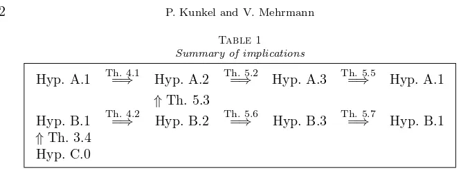
Table 1
Summary of implications
Hyp. A.1 Th. 4.1=⇒ Hyp. A.2 Th. 5.2=⇒ Hyp. A.3 Th. 5.5=⇒ Hyp. A.1
⇑Th. 5.3
Hyp. B.1 Th. 4.2=⇒ Hyp. B.2 Th. 5.6=⇒ Hyp. B.3 Th. 5.7=⇒ Hyp. B.1
⇑Th.3.4 Hyp. C.0
additional condition, see, e.g., [6]. Moreover, the consistency of the inhomogeneity can be checked numerically if one determines an approximation to the residual
r=Ex˙−Ax−f (5.45)
by using a discretized version of it. See also [6] for a similar statement.
Remark 5.9. Up to now, we have not yet addressed property 2) of Hypothe-sis A.3. This is due to the fact that it is actually implied by the other properties. Nevertheless, we have included it to make the following procedure possible. Let (E, A) satisfy Hypothesis A.3. Then there is a minimal value ˆµ, such that Hypothesis A.3 is fulfilled with ˆµreplacing k−1. Property 2) of Hypothesis A.3 then guarantees that the quantitiesaanddare uniquely fixed and that the theory concerning the reduced DAE still works for the smaller derivative arrays. If µj is the strangeness index of
(E, A) restricted toIj from (3.3) forj∈N, it is possible to show that
ˆ µ= max
j∈N{µj}. (5.46)
In particular, one can consider ˆµas a generalization of the strangeness index for such a pair (E, A). Cp. [7] in the case of regular DAEs.
6. Summary and Conclusions. We started with properties of pairs of matrix functions and the associated DAEs when they possess a well-defined strangeness in-dex. We then examined pairs of matrix functions which exhibit the same properties. In particular, the investigations ran on two levels, where in the more restrictive case additional structure of the space of consistent inhomogeneities was considered. The results of this paper are that on both levels we have obtained three equivalent char-acterizations of the corresponding class of pairs. In particular, they were by means of spaces, of canonical forms and of derivative arrays. To give an overview over all theorems that contributed to these characterizations, we first introduce the following hypothesis for completeness.
Hypothesis C.0. The pair (E, A)of matrix functions has a well-defined
strangeness index.
Table 2
Levels and equivalences
Hyp. A.1 ⇐⇒ Hyp. A.2 ⇐⇒ Hyp. A.3
⇑
Hyp. B.1 ⇐⇒ Hyp. B.2 ⇐⇒ Hyp. B.3
⇑
Hyp. C.0
(when one includes the most special level of a well-defined strangeness index) and their equivalent characterizations, see Table 2.
Of course, the most important level is the most general top level. For numerical purposes it is therefore worth mentioning that the properties of DAEs belonging to this level allow for a numerical treatment via the associated reduced problem. Overall, we have obtained classifications for several different classes of possibly over-or underdetermined DAEs.
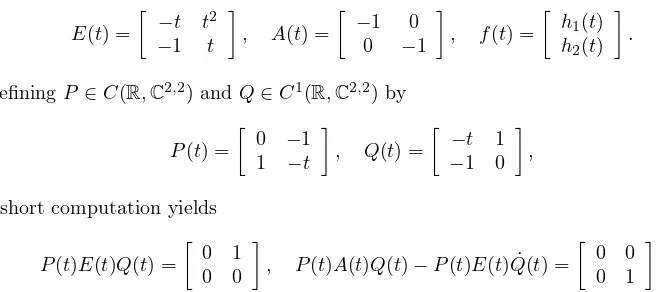
We finish up with a small example in order to illustrate the various characteri-zations we have dealt with in this paper. It should, however, be noted that such an example cannot cover all aspects we have touched here.
Example 6.1. LetE, A∈C(R,C2,2) andf ∈C(R,C2) be given by
E(t) =
−t t2
−1 t
, A(t) =
−1 0 0 −1
, f(t) =
h1(t) h2(t)
.
DefiningP ∈C(R,C2,2) andQ∈C1(R,C2,2) by
P(t) =
0 −1 1 −t
, Q(t) =
−t 1
−1 0
,
a short computation yields
P(t)E(t)Q(t) =
0 1 0 0
, P(t)A(t)Q(t)−P(t)E(t) ˙Q(t) =
0 0 0 1
.
Hence, the pair (E, A) of matrix functions has a well-defined strangeness indexµ= 1 . In particular, we have F, G∈C(R,C1,1) with F(t) = 1 and G(t) = 0 in (3.1). It is then obvious that (E, A) satisfies Hypothesis B.2.
Writing down the associated DAE (1.1) as
−tx˙1+t2x˙2=−x1+h1(t), −x˙1+tx˙2=−x2+h2(t),
we can multiply the second equation withtand subtract the so obtained relation from the first equation. This yields
We can then differentiatex1 and eliminate ˙x1in the second equation. In this way, we obtain the consistency condition
˙
h1(t)−th˙2(t) = 0,
which is certainly not of the form (3.22). To obtain all solutions of the corresponding homogeneous problem, we can choose x2 = −c with arbitrary c ∈ C1(R,C) to get x1=−tc. SplittingQaccording to (3.13), the part Φ is empty due to d= 0 and the parts Ψ,Θ are given by
Ψ(t) =
−t
−1
, Θ(t) =
1 0
.
Hence, the solution space Khas the required form (3.16). Furthermore, if the
inho-mogeneity is consistent, then the functionxdefined by
x(t) =
h1(t)−th2(t) 0
= Θ(h1(t)−th2(t))
is a particular solution of the DAE of the form (3.19). In order to show that the given pair (E, A) satisfies Hypothesis B.1, we must show that there exists a suitable matrix functionR∈C(R,C2,2) such that consistency of the inhomogeneity is characterized by a relation of the form (3.22). The property (3.20) holds here for everyRbecause ofd= 0. Choosing R=P as suggested in the general setting and transforming the original DAE by multiplying withRfrom the left gives
˙
x1−tx˙2=x2+f1(t), 0 =−x1+tx2+f2(t),
with
R(t)f(t) =
0 −1 1 −t
h1(t) h2(t)
=
−h2(t) h1(t)−th2(t)
=
f1(t) f2(t)
.
Note that the numbering of the components is here different from that in (3.21). Solving again forx1, differentiating, and eliminating ˜x1gives the consistency condition
f1(t) = ˙f2(t),
which obviously is of the form (3.22).
Turning to derivative arrays, we must considerM1, N1 due to k= 2. These are given by
M1=
−t t2 0 0
−1 t 0 0 0 2t −t t2
0 2 −1 t
, N1=
−1 0 0 0
0 −1 0 0
0 0 0 0
0 0 0 0
.
Following Hypothesis A.3, we can choose the matrix functionsZ3, T3 according to
Z3(t)H = [ 1 −t|0 0 ], T3(t) =
t 1
while all possible matricesZ4 can be obtained from the choice
Z4H=
1 −t 0 0
0 0 1 −t
by multiplying with some nonsingular matrix from the left. Recallingd= 0, the part 3) of Hypothesis A.3 is trivially satisfied. In order to show part 4) of Hypothesis B.3, we again chooseR=P. The corresponding derivative arrays are given by
˜ M2=
1 −t 0 0 0 0
0 0 0 0 0 0
0 −2 1 −t 0 0
1 −t 0 0 0 0
0 0 0 −3 1 −t 0 −2 1 −t 0 0
, N˜2=
0 1 0 0 0 0
−1 t 0 0 0 0
0 0 0 0 0 0
0 1 0 0 0 0
0 0 0 0 0 0
0 0 0 0 0 0
.
Possible choices for the matrix functions ˜Z2,Z˜3are given by
˜
Z2(t)H = [ 1 0|0 −1|0 0 ], Z˜3(t)H= [ 0 1|0 0 ].
REFERENCES
[1] S.L. Campbell. A general form for solvable linear time varying singular systems of differential equations. SIAM J. Math. Anal., 18(4):1101–1115, 1987.
[2] S.L. Campbell and L.R. Petzold. Canonical forms and solvable singular systems of differential equations. SIAM J. Algebraic Discrete Methods, 4:517–521, 1983.
[3] E. Eich-Soellner and C. F¨uhrer. Numerical Methods in Multibody Systems. B. G. Teubner Stuttgart, 1998.
[4] E. Griepentrog and R. M¨arz.Differential-Algebraic Equations and Their Numerical Treatment. Teubner Texte zur Mathematik. Teubner-Verlag, Leipzig, 1986.
[5] P. Kunkel and V. Mehrmann. Canonical forms for linear differential-algebraic equations with variable coefficients. J. Comput. Appl. Math., 56:225–259, 1994.
[6] P. Kunkel and V. Mehrmann. Generalized inverses of differential-algebraic operators. SIAM J. Matrix Anal. Appl., 17:426–442, 1996.
[7] P. Kunkel and V. Mehrmann. Local and global invariants of linear differential-algebraic equa-tions and their relation. Electr. Trans. Num. Anal., 4:138–157, 1996.
[8] P. Kunkel and V. Mehrmann. A new class of discretization methods for the solution of linear differential algebraic equations with variable coefficients. SIAM J. Numer. Anal., 33:1941– 1961, 1996.
[9] P. Kunkel and V. Mehrmann. Analysis of over- and underdetermined nonlinear differential-algebraic systems with application to nonlinear control problems. Math. Control, Signals, Sys., 14:233–256, 2001.
[10] P. Kunkel and V. Mehrmann. Differential-Algebraic Equations — Analysis and Numerical Solution. EMS Publishing House, Z¨urich, Switzerland, 2006, to appear.
[11] P. Kunkel, V. Mehrmann, and W. Rath. Analysis and numerical solution of control problems in descriptor form. Math. Control, Signals, Sys., 14:29–61, 2001.
[12] P. Kunkel, V. Mehrmann, W. Rath, and J. Weickert. GELDA: A software package for the solution of general linear differential algebraic equations. SIAM J. Sci. Comput., 18:115– 138, 1997.
[14] R. M¨arz. Solvability of linear differential-algebraic equations with properly stated leading term. Results in Mathematics, 45:88–105, 2004.
[15] S.E. Mattsson, H. Elmquist, and M. Otter. Physical system modeling with modelica. Control Engineering Practice, 6:501–510, 1998.
[16] J.W. Polderman and J.C. Willems. Introduction to Mathematical Systems Theory: A Be-havioural Approach. Springer Verlag, New York, 1998.
[17] P.J. Rabier and W.C. Rheinboldt. Classical and Generalized Solutions of Time-Dependent Linear Differential-Algebraic Equations.Linear Algebra Appl., 245:259–293, 1996. [18] W. Rulka. SIMPACK — a computer program for simulation of large-motion multibody systems.