Full Terms & Conditions of access and use can be found at
http://www.tandfonline.com/action/journalInformation?journalCode=ubes20
Download by: [Universitas Maritim Raja Ali Haji] Date: 12 January 2016, At: 23:03
Journal of Business & Economic Statistics
ISSN: 0735-0015 (Print) 1537-2707 (Online) Journal homepage: http://www.tandfonline.com/loi/ubes20
Dynamic Efficiency Estimation
Supawat Rungsuriyawiboon & Spiro E Stefanou
To cite this article: Supawat Rungsuriyawiboon & Spiro E Stefanou (2007) Dynamic
Efficiency Estimation, Journal of Business & Economic Statistics, 25:2, 226-238, DOI: 10.1198/073500106000000288
To link to this article: http://dx.doi.org/10.1198/073500106000000288
Published online: 01 Jan 2012.
Submit your article to this journal
Article views: 88
View related articles
Dynamic Efficiency Estimation: An Application
to U.S. Electric Utilities
Supawat R
UNGSURIYAWIBOONFaculty of Economics, Chiang Mai University, Chiang Mai, Thailand 50200 (supawat@econ.cmu.ac.th)
Spiro E. S
TEFANOUDepartment of Agricultural Economics and Rural Sociology, The Pennsylvania State University, 208-B Armsby, University Park, PA 16802 (spiros@psu.edu)
The shadow cost approach is developed in the context of the dynamic duality model of intertemporal decision making to formulate theoretical and econometric models of dynamic efficiency. The dynamic efficiency model is applied to a panel of 72 U.S. major investor-owned electric utilities using fossil fuel– fired steam electric power generation over the period 1986–1999. The major results show that most electric utilities underutilized fuel relative to the aggregated labor and the maintenance input, and overutilized capital in production. States adopting a deregulation plan improve the performance of utilities in terms of the technical efficiency of variable inputs.
KEY WORDS: Deregulation; Dynamic duality; Efficiency; Electricity; Shadow cost approach.
1. INTRODUCTION
Electricity deregulation and restructuring are currently on the policy agenda in many states. The basis for historical regula-tion of the electricity industries has been to deal with natural monopoly issues in the production of electricity. The first main step toward deregulation was the Public Utility Regulatory Poli-cies Act of 1978 (PURPA) passed by the U.S. Congress, which allowed independent generators to sell their electricity to utili-ties at regulated rates. In an interpretive overview of the history and patterns of regulation in the electric industry, Smith (1996) noted that regulations in early 1900s were not motivated by a consumerist response to monopoly pricing, but rather served to protect the industry from the competitive pricing that dominated at that time. Under regulation, electric utilities had a guaranteed profit for generating electricity. This led to strong incentives to overinvest in capital as well as to operate at an inefficient level of production, which is of broad interest for researchers and policymakers (Averch and Johnson 1962; Atkinson and Halvorson 1980; Crew and Kleindorfer 2002; Granderson and Linvill 2002). The level of inefficiency of electric utilities and the forces driving inefficient levels of electricity production are critical concerns. The 1992 Energy Policy Act, followed by the Federal Energy Regulatory Commission’s (FERC) Orders 888 and 889 in April of 1996, expanded PURPA’s initiative by forc-ing utilities with transmission networks to deliver power to third parties at nondiscriminatory cost-based rates. These policy ini-tiatives recognize that although electrical transmission and dis-tribution remain natural monopolies, competition in generation is possible with new technology (e.g., gas turbines) that can achieve optimal size at modest scale and with open access to transportation networks. Table 1 summarizes the roles of fed-eral and state regulators in the electricity industry. Since an open access to generation was issued by FERC in the summer of 1996, many states enacted enabling legislation or issued a reg-ulatory order to implement retail access. Retail access allows customers to choose their own supplier of energy generation services, but each state’s retail access schedule varies accord-ing to legislative mandates or regulatory orders. An overview of the status of electricity industry restructuring in each state
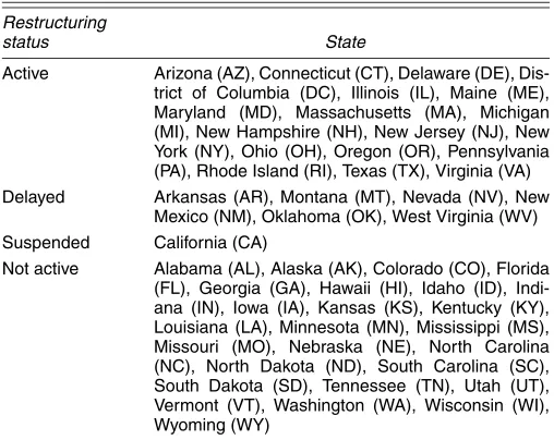
reported by the Energy Information Administration (EIA) as of March 2002 is summarized in Table 2. Twenty-five states have either enacted enabling legislation or issued a regulatory order to implement retail access. Of these states, six states have ex-perienced a delay in the restructuring process or in the imple-mentation of retail access. California is the only state in which retail access has been suspended after the energy crisis in mid-summer 2001. Twenty-six states are not actively pursuing a re-structuring plan.
Policies for open markets have led to new competitors in gen-eration and marketing, with a restructuring of the industry away from the regulated, single-provider model. Deregulation in the electricity markets has been incomplete to date, with contin-ued regulation in some segments. Under partial regulation, elec-tricity markets are not really deregulated, but are restructured. Vertical integration has diminished, and some stages of elec-tricity provision must compete in the marketplace. Deregulation of energy generation will provide important incentives for the efficient operation of electrical generators and should provide firms with incentives to lower costs by improving technical and input allocative efficiency to maximize profits. Understanding the cost structure of electric utilities in addition to other eco-nomically meaningful measurements, such as technical and al-locative efficiencies, economies of scale, and technology in the electricity industry, provides insightful information for policy makers in dealing with issues related to restructuring the elec-tricity industry.
2. BACKGROUND
Estimation of the cost structure and scale economies of elec-tric power generation in the U.S. has been studied extensively since the 1960s. Earlier studies defined various functional forms of cost functions and applied the estimation approach of the cost structure assuming that all producers operate efficiently
© 2007 American Statistical Association Journal of Business & Economic Statistics April 2007, Vol. 25, No. 2 DOI 10.1198/073500106000000288
226
Table 1. Roles of Federal and State Regulators Regulatory level Roles
Federal Regulation at the federal government level is part of the responsibility of FERC. FERC was formally known as the Federal Power Commission which was granted authority over electricity in 1935. FERC was incorporated into the newly created Depart-ment of Energy (DOE) under the current name in 1977. It has authority over interstate commerce and has been responsible for regulating the distribution and retail sales of electricity. It determines where investor-owned utilities can operate, which facilities they can construct, and at what prices they can sell. FERC also has the authority to approve or disap-prove proposed utility mergers.
State Regulation at the state government level is part of the responsibility of the state public utility com-missions (PUCs). Although FERC’s authority is ex-tensive, FERC cannot design and institute retail competition. Regulation of the retail rates paid by residential, commercial and industrial customers is carried out by the PUCs under U.S. law. The PUCs have the authority to decide whether, when and how to offer end users choice of their energy providers. The PUCs may design wholesale markets and set up organizations to manage the transmission grid in their states, but final approval of these actions re-mains with FERC.
Source: Brennan, Palmer, and Martinez (2002).
(Nerlove 1963; Christensen and Greene 1976; Considine 2000). Recent empirical applications of electric power generation re-lax this assumption to measure the inefficiency in production costs (Schmidt and Lovell 1979; Hiebert 2002). The stochastic cost frontier is applied to estimate the inefficiency level of each producer and assumes that an efficiently operating producer is represented by the estimated cost frontier. If a producer’s ob-served costs are higher than the frontier, then that deviation is attributed in part to inefficiency. A shortcoming of the stochas-tic cost frontier approach is the computational difficulties in decomposition of economic efficiency in the estimation. This shortcoming can be remedied by using stochastic estimation of the shadow cost approach. A shadow cost function is expressed in terms of shadow input prices and outputs, with shadow prices
Table 2. Status of State Electric Industry Restructuring Activity Restructuring
status State
Active Arizona (AZ), Connecticut (CT), Delaware (DE), Dis-trict of Columbia (DC), Illinois (IL), Maine (ME), Maryland (MD), Massachusetts (MA), Michigan (MI), New Hampshire (NH), New Jersey (NJ), New York (NY), Ohio (OH), Oregon (OR), Pennsylvania (PA), Rhode Island (RI), Texas (TX), Virginia (VA) Delayed Arkansas (AR), Montana (MT), Nevada (NV), New
Mexico (NM), Oklahoma (OK), West Virginia (WV) Suspended California (CA)
Not active Alabama (AL), Alaska (AK), Colorado (CO), Florida (FL), Georgia (GA), Hawaii (HI), Idaho (ID), Indi-ana (IN), Iowa (IA), Kansas (KS), Kentucky (KY), Louisiana (LA), Minnesota (MN), Mississippi (MS), Missouri (MO), Nebraska (NE), North Carolina (NC), North Dakota (ND), South Carolina (SC), South Dakota (SD), Tennessee (TN), Utah (UT), Vermont (VT), Washington (WA), Wisconsin (WI), Wyoming (WY)
Source: EIA website.
(internal to the firm) defined as input prices forcing the techni-cally efficient input vector to be the cost-minimizing solution for producing a given output. Shadow prices will differ from market (actual) prices in the presence of inefficiency.
These two approaches to measuring inefficiency arising from production cost developed under the static context are condi-tioned on some inputs, referred to as quasi-fixed inputs. Short-comings of the static approaches include ignoring the explicit role of time and also how the adjustment of quasi-fixed inputs to the observed long-run level occurs. The analysis of the tran-sition path of quasi-fixed factors toward their desired long-run levels can be remedied by explicitly incorporating costs of ad-justment for the quasi-fixed factors. The underlying idea is that the adjustment process of quasi-fixed factors generates addi-tional transition costs, and a firm’s optimal intertemporal behav-ior can be determined by appealing to the notion of adjustment costs in solving the firm’s optimization problem.
The present study incorporates adjustment costs for the quasi-fixed factors into a model of firm behavior leading the firm’s dynamic production decision problem. The static shadow cost approach is generalized using the dynamic duality model of intertemporal decision making to establish a dynamic ef-ficiency model of the cost-minimizing firm. The specific ob-jectives of this study are to estimate and decompose the cost inefficiency of U.S. electric power generation, to characterize the cost structure under dynamic adjustment, and to evaluate the performance of different electric utilities located within or outside of states with a restructuring plan.
Section 3 presents theoretical background on the economics of efficiency and dynamic factor demands. Section 4 develops the integrated theoretical and econometric models of a dynamic efficiency model. Section 5 discusses the primary sources of data used to construct the dataset and key assumptions under-lying the construction. The Section 6 presents the estimation results of the dynamic efficiency model, and Section 7 closes with some conclusions.
3. THEORETICAL FRAMEWORK
3.1 Decomposition of Economic Efficiency and Shadow Cost Approach
Consider producers facing a strictly nonnegative vector of in-put prices,w∈RN++, seeking to minimize the cost,w′x, given a nonnegative vector of input quantities, x∈RN+, which they incur in producing a nonnegative vector of outputs, y∈RM
+.
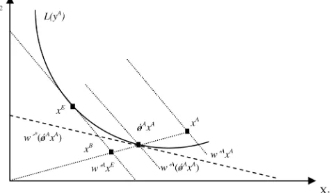
The input-oriented measurement and decomposition of cost ef-ficiency are illustrated in Figure 1. A producer uses input xA,
available at price wA, to produce output yA, which is mea-sured using IsoqL(yA). The measure of cost efficiency is given by the ratio of minimum cost C(yA,wA)=w′AxE to actual cost w′AxA. The producer’s input-oriented technical efficiency can be defined as the ratio of expenditure at w′AφAxA to ex-penditure atw′AxA. A measure of input allocative efficiency is defined as the ratio of cost efficiency to input-oriented tech-nical efficiency, (w′AxE)/(w′AφAxA). Figure 1 also illustrates how shadow prices, w∗, are input prices that make the tech-nically efficient input vectorφAxAthe minimum-cost solution for producing a given outputyA. An input-oriented measure of
Figure 1. The Input-Oriented Measurement and Decomposition of Cost Efficiency.
the technical efficiency of the producer is provided byφA<1, because y=f(φAxA). The producer is also allocatively ineffi-cient, because the marginal rate of substitution atφAxA∈L(yA)
diverges from the actual input price wA. However, the pro-ducer is allocatively efficient relative to the shadow input price,
w∗=θn1wA, where θn1 represents the values of allocative in-efficiency of variable input demands. An estimate of alloca-tive inefficiency of variable input demands>(<) 1 means that the ratio of the shadow price of the nth variable input rela-tive to the first variable input is considerably greater (less) than the corresponding ratio of actual prices. This implies that the firms are underusing (overusing) the nth variable input rela-tive to the first variable input. Following Kumbhakar and Lovell (2000), who generalized the early formulations of modeling in-efficiency in dual function given by Toda (1976) and Atkinson and Halvorson (1980), a shadow cost function is expressed in terms of shadow input prices and outputs. Given a flexi-ble functional form for specifying the shadow cost function, the stochastic shadow cost system, consisting of the producer’s observed costs and observed input demand in terms of shadow input prices and outputs, can be estimated after appending a linear disturbance into each equation.
3.2 Dynamic Duality Theory of Intertemporal Decision Making
Consider the intertemporal model in which a firm seeks to minimize the discounted sum of future production costs over an infinite horizon and holds static expectations on the set of prices and the sequence of production targets. Price expectations are static in the sense that the decision maker expects the current real prices and technology to persist indefinitely in each base period (Epstein and Denny 1983),
J
w,c,K(t),y(t)
=min
I>0 ∞
t
e−rs[w′x(s)+cK(s)]ds, (1)
subject toK˙(s)=I(s)−δK(s),K(0)=K0>0,K(s) >0, and
y(s)=F[x(s),K(s),K˙(s)], for all s∈ [t,∞), wherew is vec-tor of variable input prices,xandKare vectors of variable in-puts and quasi-fixed inin-puts, cis the vector of rental prices of quasi-fixed inputs, I and K˙ are gross and net rates of invest-ment,ris the constant discount rate,δis a constant depreciation rate,y(s)is a sequence of production targets over the planning
horizon starting at timet, andF(x(s),K(s),K˙(s))is the single-output production function. The inclusion of net investmentK˙
in the production function reflects the internal cost associated with adjusting quasi-fixed factors in terms of foregone output.
The dynamic programming equation for the problem (1) can be expressed as
rJ(w,c,K,y)
=min
x,I>0
w′x+cK+(I−δK)Jk+γy−F(x,K,K˙), (2)
whereγ≥0 is the Lagrangian multiplier associated with the production target, defined as the short-run, instantaneous mar-ginal cost (Stefanou 1989).
Epstein (1981) demonstrated that a full dynamic duality can be solved by the appropriate static optimization problem as ex-pressed in the dynamic programming equation. The result of intertemporal duality theory is that it provides readily imple-mental systems of dynamic factor demands. Differentiating the optimized version of the dynamic programming equation with respect to candwyields the optimal net investment demand and optimal variable input demand,
˙
K∗=Jkc−1(rJc−K) and
(3)
x∗=rJw−JkwK˙∗=rJw−Jkw(Jkc−1(rJc−K)).
Empirical applications of these dynamic factor demand spec-ifications have been given by Epstein and Denny (1983), Vasavada and Chambers (1986), Bernstein and Nadiri (1988), Fernandez-Cornejo, Gempesaw, Elterich, and Stefanou (1992), and Luh and Stefanou (1991, 1996).
4. SPECIFICATION OF DYNAMIC EFFICIENCY MODEL
4.1 Dynamic Efficiency Model Derivation
Here the static shadow cost model presented in Section 3.1 is generalized using the dynamic duality model of intertempo-ral decision making presented in Section 3.2. In the presence of allocative and technical inefficiencies in the production func-tion, the behavioral value function of the dynamic programming equation for a firm’s intertemporal cost minimization behav-ior in the presence of technical change that corresponds to the shadow prices and quantities can be expressed in the form of a behavioral Hamiton–Jacobi equation,
rJb(wbnit,cit,Kit,yit,tit)
=(wbnit)′xbnit+cit′Kit+ ˙Kitb′(Jkb,it)
+γnb
yit−F(xbnit,Kit,K˙itb,tit)+Jtb,it, (4)
whereJkb,it =∂Jitb/∂K and Jtb,it =∂Jbit/∂t; n=1, . . . ,N is an index of variable inputs; i=1, . . . ,I is an index of firms;
t=1, . . . ,T is an index of time periods; c is the user cost of capital;K is a quasi-fixed input of capital stock; y is the output; t is time trend; wb=(λ1w1, . . . , λNwN), withλn>0
representing the behavioral prices of variable inputs;λnis the
allocative inefficiency parameters for the nth variable input;
wnis the observednth variable input price;Jkb=µJkarepresents
the marginal behavioral value of capital, whereJka represents
the observed marginal value of capital andµ is the allocative inefficiency parameter of net investment;xb=(1/τx)x
repre-sents the behavioral variable inputs, whereτx≥1 is the inverse
of producer-specific scalars providing input-oriented measures of the technical efficiency in variable input use and x is the observed variable input use;K˙b=(1/τk)K˙ represents the
be-havioral net investment level, where τk ≥1 is the inverse of
producer-specific scalars providing input-oriented measures of the technical efficiency in net investment andK˙ =dK/dtis the level of net investment; andγb≥0 is the behavioral Lagrangian multiplier defined as the short-run, instantaneous marginal cost. If thenth variable input is allocatively efficient, thenλn=1.
The values ofλn>1 (or <1) imply that the decision maker,
ceteris paribus, allocates less (or more) of thenth input com-pared with the cost-minimizing allocation. By specifying the first variable input price as the numeraire, the prices of variable inputs demands are redefined aswbnit=(λn/λ1)wnit=θn1iwnit,
wheren=1, . . . ,Nandθ11i=1. The values of allocative
effi-ciency of variable inputs demands,θn1i, represent price
distor-tions of thenth variable input relative to the first variable input. An estimate of allocative efficiency of variable inputs demands greater (less) than 1 means that the ratio of the shadow price of thenth variable input relative to the first variable input is con-siderably greater (less) than the corresponding ratio of actual prices. This implies that the firms are underusing (overusing) thenth variable input relative to the first variable input.
Without the notation of the indices of variable inputs, firms, and time periods, the behavioral value function of the dynamic programming equation in (4) using the basic idea underly-ing the input-oriented efficiency measurement approach can be rewritten in terms ofJb(λw,c,K,y,t)as
rJb(λw,c,K,y,t)=(λw)′xb+c′K+ ˙Kb′Jbk(·)
+γb
y−F(xb,K,K˙b,t)
+Jtb(·). (5) Differentiating (5) with respect tocand(λw)yields the optimal investment demand
rJcb(·)=K+ ˙Kb′Jkcb(·)+Jtcb(·) or
(6)
˙
Kb(·)=(Jbkc(·))−1rJcb(·)−K−Jtcb(·)
and optimal variable input demand
rJb(λw)(·)=xb+ ˙Kb′Jkb(λw)(·)+Jtb(λw)(·) or
(7)
xb(·)=(λ)−1
rJwb(·)− ˙Kb′(·)Jkwb (·)−Jtwb(·)
.
In the presence of technical inefficiency of net investment and variable inputs, the corresponding observed investment and variable input demands using the input-oriented approach can be written in terms of the optimal investment and variable input demands as The dynamic programming equation for the firms’ intertem-poral cost-minimization behavior corresponding to the actual prices and quantities can be expressed as
rJa=w′x+c′K+ ˙K′Jka+γa
y−F(xb,K,K˙b,t)
+Jta, (10)
where input-oriented efficiency measurement is maintained. Considering the actual quantities as the optimal levels, the op-timized actual quantities are K˙o=τkK˙b(·) and xo=τxxb(·).
The optimized actual dynamic programming equation can be expressed as
rJa=w′xo+c′K+ ˙Ko′Jak+Jta, (11) whereJka=(1/µ)Jkb(·), implying that the marginal behavioral value of capital diverges from the marginal actual value of cap-ital byµand assuming that a shift in the behavioral value func-tion is the same proporfunc-tion as the actual value funcfunc-tion so that
Jta=Jtb(·). The optimized actual value function can be rewrit-ten in the terms of the behavioral value function as
rJa=w′(τx/λ)rJwb(·)− ˙K b′
(·)Jkwb (·)−Jtwb(·)
+c′K+(τkK˙b(·))(Jkb(·)/µ)+Jtb(·). (12)
Differentiating (11) with respect tocandw, the optimized ac-tual investment demand yields
rJca=K+ ˙Ko′Jkca +Jtca or
(13)
˙
Ko=(Jkca)−1(rJca−K−Jtca),
and the optimized actual variable input demand yields
rJaw=xo+ ˙Ko′Jakw+Jtwa or
(14)
xo=rJwa− ˙Ko′Jkwa −Jatw.
Differentiating (12) with respect to c and substituting into (13), the optimized actual investment demand in terms of the behavioral value function yields (up to second-order terms)
Note that third-order terms involving the derivative ofJb(·)
with respect to(w,c,k)and(w,c,t)are ignored.
Differentiating (12) with respect to w and substituting into (14), the optimized actual variable input demand in terms of the behavioral value function yields (up to second-order terms)
xo=r
− ˙Ko
The behavioral conditional demand for the numeraire vari-able input is derived by rearranging the behavioral-optimized value function of the dynamic programming equation (5) as
rJb=xbn+wbxb(·)+cK+ ˙Kb(·)Jkb+Jtb, (17) wherexbn is the behavioral demand for the numeraire variable input andxbis the behavioral demand for the other variable in-puts, leading to the behavioral conditional demand for the nu-meraire variable input defined as
xbn(·)=rJb−wbxb(·)−cK− ˙Kb(·)Jkb−Jtb. (18) The optimized actual demand for the numeraire variable input is
xon=τxxbn(·)=τx{rJb−wbxb(·)−cK− ˙Kb(·)Jkb−Jbt}. (19)
The optimal investment demand function for the single quasi-fixed factor case in (6) (Treadway 1971, 1974) can be expressed as a univariate linear accelerator,
˙
Kit∗(wb,c,K,y,t)= ˙Kitb(·)=M
Kit−Kit∗(wb,c,y,t)
, (20) whereMis the partial adjustment coefficient that indicates how quickly the current level of capital stock,Kit, will adjust to the optimal capital stock levels,Kit∗.
With a single quasi-fixed input of capital stock, the behav-ioral value function taking the quadratic functional form and assuming symmetry of the parameters where Aij=Ajican be specified as
The producer- and input-specific estimates of technical and allocative efficiencies must be specified to implement the dy-namic efficiency model in the panel data context. Following Cornwell, Schmidt, and Sickles (1990), the allocative and tech-nical efficiencies of net investment and variable inputs are specified as producer-specific and time-varying–specific para-meters. The allocative and technical efficiencies of net invest-ment and variable inputs are guaranteed to be nonnegative using the exponential transformation. All coefficient parameters for the system equation of the dynamic efficiency model can be es-timated after appending a linear disturbance vector with mean vector 0 and variance–covariance matrixto the system equa-tion. Joint estimation of the system equation provides parameter
estimates of the behavioral value function represented by (21). Appendix A presents the specification for the system equation of the dynamic efficiency model consisting of the optimized actual demand for net investment and variable inputs in terms of the parameter estimates expressed in (21). The net invest-ment equation conforms to the linear accelerator in (20), where
[r−(Ack)−1]is the adjustment rate per annum.
The maintained model is recursive in the endogenous able of net investment demand, serving as an explanatory vari-able in the varivari-able input demand equations. The estimation can be accomplished in two stages. In the first stage, the net investment demand is estimated using maximum likelihood (ML) estimation. In the second stage, because the variable in-put demand equations are overidentified, the system of vari-able input demand equations is estimated using generalized method-of-moments (GMM) estimation given all parameter values obtained in the first stage. All predetermined variables, including exogenous and dummy variables of each equation in the variable input demand equations, are defined as the instrumental variables of the system equation in the second stage. One function of GMM estimation is to find instrumen-tal variables,z, that are correlated with exogenous variables in the model but uncorrelated with the residual,ε, implying the orthogonality conditions, E(z′ε)=0. If the disturbances are heteroscedastic and serially correlated, then estimation in the presence of heteroscedasticity and autocorrelation can be cor-rected by applying a flexible approach developed by Newey and West (1987). The number of autocorrelation terms used in com-puting the covariance matrix of the orthogonality conditions can be determined by the procedure of Newey and West (1994).
5. DISCUSSION OF DATA
In this study data on fossil fuel–fired steam electric power generation for major investor-owned U.S. utilities are used to construct a dataset because these are the dominant sectors of the U.S. electricity industry. Approximately 61% of all the electric-ity supplied by the U.S. electric power industry in 1999 came from fossil fuel–fired steam turbines. Investor-owned utilities own 71% of the U.S. generating capacity owned by both util-ities and nonutility generators and are responsible for 74% of all retail sales of electricity. The primary sources of data are the EIA, the FERC, and the Bureau of Labor Statistics (BLS). The definitions of the data used in this study are summarized next.
The output variable,yit, is represented by net steam electric
power generation in megawatt-hours defined as the amount of power produced using fossil fuel–fired boilers to produce steam for turbine generators during a given time period. Net steam electric power generation for each time period is reported by firm in the EIA’s Form 1.
The price of fuel aggregate,w1it, is a price index of fuels (i.e.,
coal, oil, gas) calculated as
w1it+1
fuel (i.e., coal, oil, gas) from the EIA’s Form 423 of firmiat
timet, and Qfit is the consumption of the same fuel from the
EIA’s Form 423 of firmiat timet.
The quantity of fuel,x1it, is calculated as the steam power
production fuel costs reported by firm in the EIA’s Form 1, di-vided by the price of fuel aggregate.
The price of labor and maintenance aggregate,w2it, is a cost
share–weighted price index for labor and maintenance. The price of labor is a firm-level average wage rate. Data on a firm’s wage rate and number of employees are reported in the EIA’s Form 1. The price of maintenance and other supplies is an industry-level price index of electrical supplies from the BLS. The average weight of the labor cost amounts to 30% of nonfuel variable costs over the study period.
The quantity of labor and maintenance,x2it, is measured as
the aggregate costs of labor and maintenance divided by the price index for labor and maintenance. Data on labor and main-tenance costs are calculated by subtracting fuel expenses from total steam power production expenses reported in the EIA’s Form 1.
The price of capital,cit, is the yield of the firm’s latest issue
of long-term debt adjusted for appreciation and depreciation of the capital goods using the Christensen and Jorgenson (1970) cost of capital formula,
cit=pkt[idit+sit(reit−idit)+d−ft], (23)
wherepkt is a price index for electrical generating plants and equipment from the BLS;idit is the adjusted corporate bond
rate from the Federal Reserve Board, adjusted by firm based on its bond ratings by Moody’s Investor Service reported by the EIA’s Form 1; sit is the equity share of total capital, defined
as total proprietary capital (TPC) divided by the sum of total proprietary capital and total long-term debt (TOTB);reit is the
equity rate of return, defined as the ratio of net income to total proprietary capital;dis a depreciation rate assuming 30 years of straight-line depreciation; andftis the inflation rate, which is
the rate of changing in overall wholesale prices reported by the BLS. Data on TPC, TOTB, and net income are obtained from the EIA’s Form 1.
The values of capital stocks are calculated by obtaining the valuation of base and peak load capacity at replacement cost to estimate capital stocks in a base year and then updating it in subsequent years based on the value of additions to and retire-ments of steam power plants, as discussed by Considine (2000). The base year capacity is calculated by multiplying the price of new generation capacity in dollars per megawatt(PNGit) re-ported in the EIA’s Form 1 and the base year nameplate capacity in megawatts(CAPit)reported in the EIA’s Form 759,
Kit=PNGit·CAPit, t=1986. (24)
For subsequent years, the values of capital stocks are calcu-lated by
Kit=
(1−d)(Kit−1)pkit
pkit−1
+Ait−Rit, t=1987, . . . ,1999,
(25)
where d denotes the depreciation rate assuming 30 years of straight-line depreciation;Kit is equal to the nominal stock di-vided by the price index for electrical generating plants and equipment,pkit; andAitandRit denote additions to and
retire-ments of steam power plants reported in the EIA’s Form 1. The total cost for steam electric power generation, TCit, is
defined as the sum of the product of input prices and quanti-ties for aggregate fuel, aggregate labor, and maintenance and capital,
TCit=
2
n=1
wnitxnit+citKit. (26)
Initially, all of these data sources were combined to construct a dataset from the variables for 110 electric utilities with all variables defined for the time period 1986–1999. Electric utili-ties that are subsidiaries of holding companies were aggregated into one entity. Christensen and Greene (1976) showed that a failure to recognize holding companies leads to underestima-tion of scale economies. Once the holding companies that have generating plants located in states with and without the dereg-ulation plan were excluded, the remaining 72 electric utilities composed the panel used in this study. These are divided into two groups according to the status of state electric industry re-structuring activity. Electric utilities in group A have all plants located in states that enacted enabling legislation or issued a regulatory order to implement retail access; those in group B have all plants located in states without the deregulation plan. The final set the panel data on 72 electric utilities over the pe-riod 1986–1999 is used in this study. Table 3 summarizes the data used in this study. The observed shares are 57% by fuel, 16% by labor and maintenance, and 27% by capital. A list of the electric utilities presented in Appendix B.
6. EMPIRICAL RESULTS
The dynamic efficiency model accounts for four inefficiency parameters: technical and allocative inefficiencies in net invest-ment and variable input demands. Technical inefficiency of net investment,τk, is represented by the physical operation of
gen-erating plants. Thermal conversion efficiency is used to measure the performance of generating plants. The EIA report showed
Table 3. Data Summary for 72 Electric Utilities Over the Periods 1986–1999
Variable Units Mean SD Minimum Maximum
Output,y (×106MWhr) 13.643 12.152 .499 79.723
Fuel,x1 (×106dollars) 254.411 246.604 19.380 1,615.651
Labor and maintenance,x2 (×106dollars) 72.351 67.464 1.840 556.601
Capital,K (×106dollars) 894.768 786.477 26.148 3,878.295
Fuel price,w1 1.011 .151 .567 1.881
Labor and maintenance price,w2 1.000 .174 .568 2.798
User costs of capital,c .136 .027 .012 .272
Total cost,TC (×106dollars) 451.045 390.902 11.123 2,339.045
that the standard deviation of an average plant efficiency of steam electric power generating plants measured by thermal conversion efficiency is very low for each plant. This effect is even smaller when the firm data are used. An additional as-sumption that technical efficiency in net investment demand is constant among electric utilities is assumed. While this assump-tion permits estimaassump-tion of the system, it is also not as restrictive in this context as it may first appear. Further, a sensitivity analy-sis on the technical efficiency parameter of net investment was performed by varying the technical efficiency parameter of net investment between .60 and 1.00. The likelihood and R2 for each estimated equation are quite stable within this range and suggest no statistically significant change between the model withτk=1 andτkequal to any other value less than unity.
Al-thoughτkis firm and time-invariant, its value on average should
signal an alert concerning the potential misspecification of per-fect technical efficiency in net investment. This statistical result along with the EIA report showing that the low standard de-viation of an average plant efficiency of steam electric power generating plants measured by thermal conversion efficiency suggests the assumption thatτk=1 is a tolerable one.
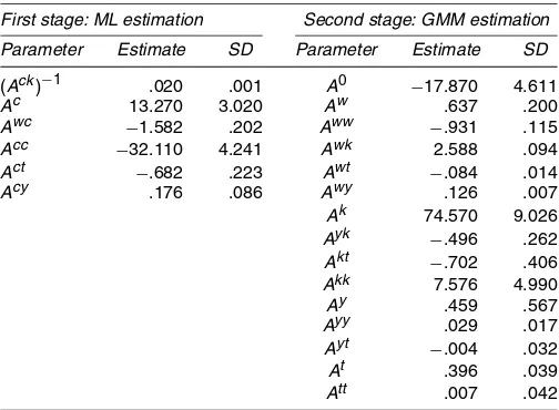
Table 4 gives the estimated coefficients and standard errors for the structural parameters of the dynamic efficiency model under the assumption that firms are perfectly technical efficient in net investment demand using ML and GMM estimations, assuming a constant real interest rate of 5%. The full set of estimated coefficients, including the dummy variables used to calculate the allocative inefficiency parameters of variable in-puts and net investment demands and the technical inefficiency parameter of variable input demand, are available from the au-thors on request. All estimated parameters from the ML estima-tion are significant at the .05 level using a two-tailed test. The log-likelihood andR2values for the net investment equation are 3,224 and .250. A lag of two periods of autocorrelation terms is used to compute the covariance matrix of the orthogonality con-ditions for the GMM estimation. The computedR2 values for the fitted quantity equations for fuel and the aggregate of labor and maintenance are .976 and .951. The test of overidentify-ing restrictions from GMM estimation usoveridentify-ing the Hansen (1982)
Jtest is significant. The null hypothesis fails to reject, imply-ing that the additional instrumental variables are valid, given
Table 4. Estimated Structural Coefficients, 1986–1999 First stage: ML estimation Second stage: GMM estimation Parameter Estimate SD Parameter Estimate SD
(Ack)−1 .020 .001 A0 −17.870 4.611
Ac 13.270 3.020 Aw .637 .200
Awc −1.582 .202 Aww −.931 .115
Acc −32.110 4.241 Awk 2.588 .094
Act −.682 .223 Awt −.084 .014
Acy .176 .086 Awy .126 .007
Ak 74.570 9.026
Ayk −.496 .262
Akt −.702 .406
Akk 7.576 4.990
Ay .459 .567
Ayy .029 .017
Ayt −.004 .032
At .396 .039
Att .007 .042
that a subset of the instrumental variables is valid and exactly identifies the coefficient.
Table 5 presents average firm allocative and technical effi-ciencies of net investment and variable input demands by all electric utilities and the group of electric utilities affected by the deregulation plan over the period 1986–1999. The technical efficiency parameter of net investment is assumed to be unity. The allocative efficiencies of net investment range from .200 for Pacific Gas & Electric Co. (CA) to 1.218 for Montana Power Co. (MT), with an average of .594. The estimated value of the allocative efficiency of net investment is<1, implying that firms are overutilizing the net investment. The estimated tech-nical efficiencies of variable inputs range from .241 for Texas Utility Electric Co. (TX) to .991 for Rochester Gas & Electric Corp. (NY), with an average of .767. By specifying the aggre-gate prices of labor and maintenance as the numeraire, the esti-mated allocative efficiencies of variable inputs range from .084 for Montana Power Co. (MT) to 6.464 for Gulf State Utilities Co. (TX), with an average of 3.105. The values of allocative efficiency of variable input demands represent price distortions of fuel relative to the aggregate of labor and maintenance. An estimated allocative efficiency of variable input demands>1 means that the ratio of the shadow price of fuel relative to that of the labor and maintenance aggregate is considerably greater than the corresponding ratio of actual prices, implying that the firms are underutilizing fuel relative to the aggregate of labor and maintenance. The estimated results indicate that all elec-tric utilities in this study except two firms, Montana Power Co. (MT) and Southern Indiana Gas & Electric Co. (IN), underuti-lized fuel relative to the aggregate of labor and maintenance. Moreover, all electric utilities in this study overutilized net in-vestment except by one firm, Montana Power Co. (MT). These results indicate that electric utilities located in states with a deregulation plan have an average firm technical efficiency of variable inputs lower than electric utilities located outside of states with the deregulation plan. This result suggests that elec-tric utilities with relatively high technical inefficiency in states adopting a deregulation plan improve the performance of their electric utilities. Furthermore, electric utilities located in states with a deregulation plan have average firm allocative efficien-cies of variable inputs and of net investment lower than those located outside of states with a deregulation plan. These results imply that electric utilities located in states with a deregulation plan are underutilizing fuel relative to the aggregate of labor and maintenance less than those located outside of states with a deregulation plan and overutilizing net investment relative to those located outside of states with a deregulation plan. How-ever, the magnitudes of the differences of allocative efficiencies of variable inputs and net investment by the group of electric utilities affected by a deregulation plan are not dramatic.
Table 5 also presents average firm allocative and technical efficiencies of net investment and variable input demands by all electric utilities and the group of electric utilities affected by a deregulation plan for separate periods during the period 1986–1999. These results allow us to examine the impact of the Energy Policy Act and the FERC Orders to a electric utility’s efficiency. Our findings indicate that electric utilities located in and outside states with a deregulation plan are overutiliz-ing net investment over the time period but are underutilizoverutiliz-ing
Table 5. Average Firm Allocative and Technical Efficiencies of Net Investment and of Variable Inputs, Given Firms Are Perfectly Technical Efficient in Net Investment, 1986–1999
Electric utility group∗efficiency scores 1986–1991 1992–1995 1996–1999 1986–1999
All electric utilities
Allocative inefficiency of net investment .759 .591 .431 .594
Technical inefficiency of variable input .754 .770 .775 .767
Allocative inefficiency of variable input 3.888 3.027 2.400 3.105
Electric utilities group A
Allocative inefficiency of net investment .752 .579 .435 .589
Technical inefficiency of variable input .708 .729 .737 .725
Allocative inefficiency of variable input 3.926 2.936 2.333 3.065
Electric utilities group B
Allocative inefficiency of net investment .802 .603 .428 .611
Technical inefficiency of variable input .801 .811 .814 .809
Allocative inefficiency of variable input 3.850 3.136 2.468 3.151
∗Group A refers to electric utilities located within of states with the deregulation plan, group B refers to electric utilities located outside of states with
the deregulation plan.
fuel less relative to the aggregate of labor and maintenance over the time period. Furthermore, electric utilities located in and outside states with a deregulation plan have an improved aver-age technical efficiency of variable inputs over the time period. Electric utilities located in states with a deregulation plan have higher increases of average technical efficiency of variable in-puts than those located outside states with a deregulation plan. These results imply that the Energy Policy Act and the FERC Orders result in an increase of allocative and technical efficien-cies of variable inputs for both electric utilities located in and outside states with a deregulation plan, but lead to a decrease of allocative efficiency of net investment. The federal legisla-tive initialegisla-tives promoting deregulation of the industry resulting in unprecedented wave of mergers, acquisitions, and sales of power generation plants lead to overutilization of net invest-ment of electric utilities in the industry.
The adjustment rate of capital,[r−(Ack)−1], is 3.00%, im-plying that the capital stock adjusts 3% per annum to the long-run equilibrium levels. This sluggish adjustment of cap-ital results from the nonstorable characteristic of electricity and capital-specific nature of utility investments and magnitude of the investment. Most electric utilities will choose to buy power externally to meet additional demand in the shortrun rather than build new generating plants, because prices in the wholesale market for electricity are usually not much higher than the mar-ginal cost of generating electricity by the electric utilities in the shortrun.
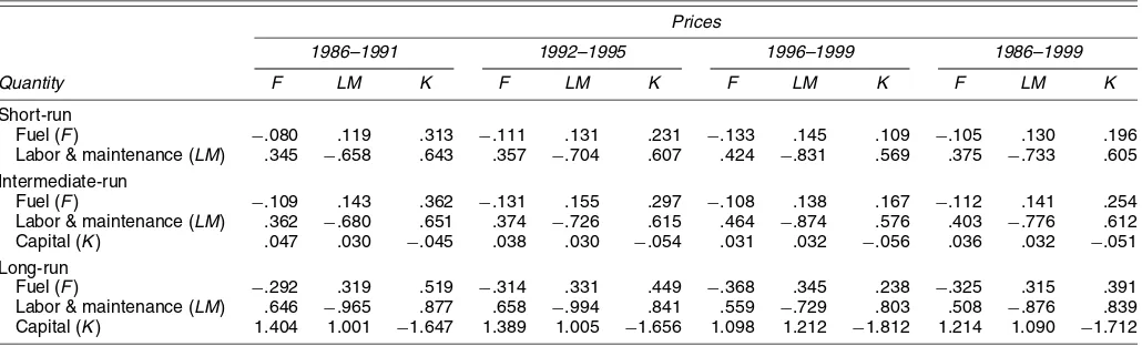
Table 6 reports weighted-average estimates of short-, inter-mediate-, and long-run input price elasticities evaluated at the long-run equilibrium level for separate periods during the pe-riod 1986–1999. Derivations of input demand elasticities are presented in Appendix C. All own-price elasticities have the expected negative sign. Overall, the estimated results of input demand elasticities do not change significantly in magnitude in each period. The magnitude of the short-run own price elastic-ity of demand for fuel indicates that it is price-inelastic. The short-run own price elasticity of demand for the aggregate of labor and maintenance is larger in absolute magnitude than that for fuel. The cross-price elasticity estimates suggest that fuel, capital, and the aggregate of labor and maintenance are substi-tutes. The magnitude of the intermediate-run elasticity changes from the short-run elasticities is not significant because of the low adjustment rate of capital stock to its long-run equilibrium level. The long-run own price elasticities of demand for fuel and the aggregate of labor and maintenance are larger in ab-solute magnitude than the short-run own price elasticities. The magnitude of the long-run own price elasticity of capital indi-cates that it is significantly price-elastic. The cross-price elas-ticity estimates suggest that fuel, capital, and the aggregate of labor and maintenance are substitutes, and the relatively large cross-price elasticities suggest the significant substitution possi-bilities among these inputs. The estimated results of own-price elasticities of input demand for separate periods imply that the Energy Policy Act and the FERC Orders result in more price
Table 6. Short-Run, Intermediate-Run, and Long-Run Elasticities Over the Period 1986–1999 Prices
1986–1991 1992–1995 1996–1999 1986–1999 Quantity F LM K F LM K F LM K F LM K
Short-run
Fuel (F) −.080 .119 .313 −.111 .131 .231 −.133 .145 .109 −.105 .130 .196
Labor & maintenance (LM) .345 −.658 .643 .357 −.704 .607 .424 −.831 .569 .375 −.733 .605 Intermediate-run
Fuel (F) −.109 .143 .362 −.131 .155 .297 −.108 .138 .167 −.112 .141 .254
Labor & maintenance (LM) .362 −.680 .651 .374 −.726 .615 .464 −.874 .576 .403 −.776 .612
Capital (K) .047 .030 −.045 .038 .030 −.054 .031 .032 −.056 .036 .032 −.051
Long-run
Fuel (F) −.292 .319 .519 −.314 .331 .449 −.368 .345 .238 −.325 .315 .391
Labor & maintenance (LM) .646 −.965 .877 .658 −.994 .841 .559 −.729 .803 .508 −.876 .839 Capital (K) 1.404 1.001 −1.647 1.389 1.005 −1.656 1.098 1.212 −1.812 1.214 1.090 −1.712
elastic for fuel, the aggregate of labor and maintenance, and capital. Furthermore, the estimated results of cross-price elas-ticities of input demand for separate periods suggest that the impact of the Energy Policy Act has generally increased the substitution possibilities between fuel and the aggregate of la-bor and maintenance and has decreased the substitution possi-bilities between fuel and capital in every period. The impact of the FERC Orders on the substitution possibilities among inputs provides mixed effects. Further, the Morishima elasticities of substitution (MES), which measure the relative adjustment of factor quantities when a single factor price changes, are com-puted to examine the substitution possibilities among inputs be-tween different time periods.
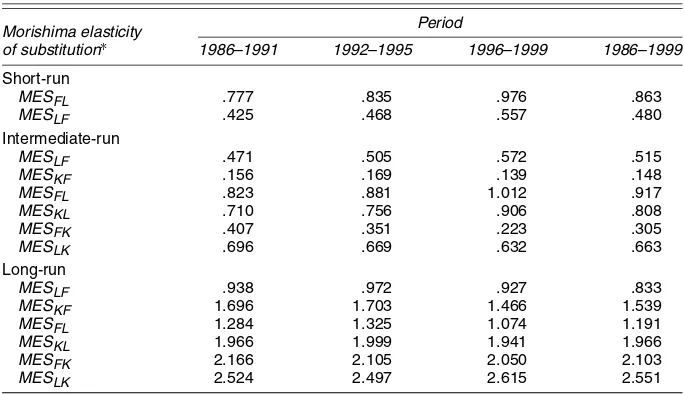
Table 7 reports weighted-average estimates of short-, inter-mediate-, and long-run MES for separate periods during the period 1986–1999. Derivations of MES are also presented in Appendix C. The estimated MES of fuel for the aggregate of labor and maintenance is greater than that of the aggregate of labor and maintenance for fuel in every time period. The re-sults of the intermediate- and long-run periods indicate that the estimated MES of fuel for capital is greater than that of capi-tal for fuel. The estimated MES of capicapi-tal for the aggregate of labor and maintenance is greater than that of the aggregate of labor and maintenance for capital in the intermediate run but shows an opposite effect in the long run. In the short run, the estimated results of MES suggest that the impacts of the En-ergy Policy Act and the FERC Orders lead to an increase of the MES between fuel and the aggregate of labor and maintenance. In the intermediate run, the results indicate that the Energy Pol-icy Act leads to an increase in capital and the aggregate of labor and maintenance relative to an increase of fuel prices and an in-crease in fuel and capital relative to an inin-crease of the aggregate of labor and maintenance prices, but a decrease in fuel and the aggregate of labor and maintenance relative to an increase in capital prices. The impact of the FERC Orders shows that the aggregate of labor and maintenance increases, whereas capital decreases relative to an increase in fuel prices. Fuel and capi-tal increase relative to an increase in the aggregate of labor and
maintenance prices. Fuel and the aggregate of labor and main-tenance decrease relative to an increase of capital prices. In the long run, the impact on the Energy Policy Act leads to an in-crease in capital and the aggregate of labor and maintenance relative to an increase in fuel prices and an increase in fuel and capital relative to an increase in the aggregate of labor and maintenance prices but leads to a decrease in fuel and the aggre-gate of labor and maintenance relative to an increase in capital prices. The impact on the FERC Orders shows that the aggre-gate of labor and maintenance and capital decrease relative to an increase in fuel prices, fuel and capital decrease relative to an increase in the aggregate of labor and maintenance prices, and in fuel decreases but the aggregate of labor and maintenance increases relative to an increase in capital prices.
The estimated optimal capital stocks are calculated and com-pared with the actual capital stocks to account for the capacity utilization, which provides some insight into the efficiency of capital use by a firm. Values of the ratio of optimal capital to actual capital stocks<1 imply that a firm is overutilizing capi-tal, whereas values>1 imply that a firm is underutilizing cap-ital. Figure 2 shows the distribution of the ratio of capital by firm. There are 46 firms with values of the ratio of capital be-low the average. The estimated results indicate that all electric utilities in this study except three firms [Kansas Gas & Elec-tric Co. (KS), The Detroit Edison Co. (MI), and Texas Utilities Electric Co. (TX)] are overcapitalized.
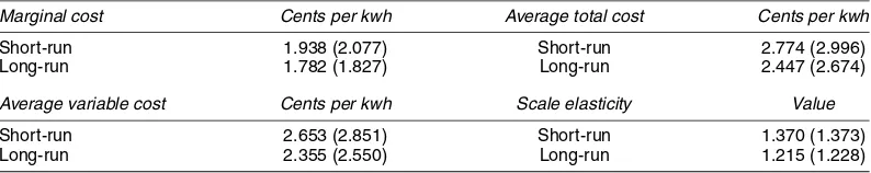
Table 8 presents weighted-average estimates of the short-and long-run marginal cost, average variable cost, average total cost, and scale elasticity for both the prederegulation (1986–1996) and the combined prederegulation and postdereg-ulation (1986–1999) periods. Derivation of scale elasticity is presented in Appendix D. The short-run scale elasticity is de-fined as the ratio of short-run average variable cost to short-run marginal cost, whereas the long-run scale elasticity is defined as the ratio of long-run average variable cost to short-run mar-ginal cost (Stefanou 1989). Scale elasticity values<1 imply de-creasing returns to scale, whereas values>1 imply increasing returns to scale. Overall, the estimates of the prederegulation
Table 7. Short-Run, Intermediate-Run, and Long-Run Morishima Elasticities of Substitution (MES) Over the Period 1986–1999
Morishima elasticity of substitution∗
Period
1986–1991 1992–1995 1996–1999 1986–1999
Short-run
MESFL .777 .835 .976 .863
MESLF .425 .468 .557 .480 Intermediate-run
MESLF .471 .505 .572 .515
MESKF .156 .169 .139 .148
MESFL .823 .881 1.012 .917
MESKL .710 .756 .906 .808
MESFK .407 .351 .223 .305
MESLK .696 .669 .632 .663
Long-run
MESLF .938 .972 .927 .833
MESKF 1.696 1.703 1.466 1.539
MESFL 1.284 1.325 1.074 1.191
MESKL 1.966 1.999 1.941 1.966
MESFK 2.166 2.105 2.050 2.103
MESLK 2.524 2.497 2.615 2.551
∗SubscriptF=fuel;L=labor and maintenance;K=capital.
Figure 2. Distribution of the Ratio of Optimal Capital to Actual Capital.
period are consistent with those of the combined prederegula-tion and postderegulaprederegula-tion period. The estimates of short- and long-run marginal costs are 2.077 and 1.827 cents per kwh for the prederegulation period and 1.938 and 1.782 cents per kwh for the combined prederegulation and postderegulation pe-riod. In addition, the estimates of short- and long-run average total costs are 2.996 and 2.674 cents per kwh for the pred-eregulation period and 2.774 and 2.447 cents per kwh for the combined prederegulation and postderegulation period. These results support the hypothesis that the deregulation of energy generation can provide important incentives for the efficient operation of electrical generators by lowering costs to maxi-mize profits. The estimate of scale elasticity measure indicates increasing returns to scale in the industry prederegulation and postderegulation. However, the estimates for the prederegula-tion period indicate higher increasing returns to scale in the industry than those for the combined prederegulation and post-deregulation period.
7. CONCLUSIONS
This study addresses the evolution of the structure of elec-tricity production as the industry faces deregulation using a structured economic model of dynamic production. The sta-tic shadow price approach and the dynamic duality model of intertemporal decision making are integrated to formalize the theoretical and econometric models of dynamic efficiency for cost-minimizing firms. The results indicate that most electric utilities in this study underutilized fuel relative to the aggre-gate of labor and maintenance and overutilized net investment. The results suggests that electric utilities with relatively high technical inefficiency in production located in states that have adopted a deregulation plan improve their performance. The
magnitudes of the difference of allocative efficiencies of vari-able inputs and net investment by a group of electric utilities affected by a deregulation plan are not significant. The esti-mates of the short-, intermediate-, and long-run input price elas-ticities indicate the substitution possibilities among the inputs. Most electric utilities in this study had optimal capital below actual capital stocks, implying that most electric utilities are overcapitalized in the production. The estimates of short- and long-run average (marginal) costs for the prederegulation pe-riod are higher than those for the combined prederegulation and postderegulation period. These results suggest that the deregu-lation of energy generation will provide important incentives for the efficient operation of electrical generators, and present firms with an incentive to lower costs to maximize their prof-its. The estimate of scale and elasticity measures indicates sup-porting evidence of increasing returns to scale in the industry prederegulation and postderegulation. However, the estimates for the prederegulation period suggest higher increasing returns to scale in the industry than those for the combined prederegu-lation and postdereguprederegu-lation period.
ACKNOWLEDGMENTS
The authors would like to thank an Associate Editor, two anonymous referees, Tim Considine, and Ted Jaenicke for their helput comments.
APPENDIX A: SPECIFICATION OF NET INVESTMENT AND VARIABLE INPUTS DEMANDS EQUATIONS IN
TERMS OF THE PARAMETER ESTIMATES
The system equation of the dynamic efficiency model con-sists of the optimized actual demand for net investment and variable inputs. The optimized actual investment demand de-rived using the behavioral conditional demand as expressed in (8) can be written in terms of the parameter estimates as
˙
Ko=τk(Ack)−1r(Ac+Awcwb+Accc+AckK
+Actt+Acyy)−K−Act
. (A.1) The optimized actual demand for the variable input demand equation presented in (16) is written in terms of the parameter estimates as
xo=rτx
Aww−
AwkAcc
Ack
wb
+(Aw+Awwwb+Awcc+AwkK+Awtt+Awyy)
Table 8. Short- and Long-Run Scale and Cost Elasticities for the Period 1986–1999
Marginal cost Cents per kwh Average total cost Cents per kwh
Short-run 1.938 (2.077) Short-run 2.774 (2.996)
Long-run 1.782 (1.827) Long-run 2.447 (2.674)
Average variable cost Cents per kwh Scale elasticity Value
Short-run 2.653 (2.851) Short-run 1.370 (1.373)
Long-run 2.355 (2.550) Long-run 1.215 (1.228)
NOTE: Estimated values for the prederegulation periods of 1986–1996 are in parentheses.
+1
r Awk
Ack
+1
r
AwkAct
Ack
−
Awk
Ack
(Ac+Awcwb+Accc+AckK+Actt+Acyy)
−1
r
Awt−
AwkAct
Ack
−
Awt
r
− 2
r2 Awk
Ack
˙
Ko
−
τ k
µ
Awk
Ack
K
−r Awc
Ack
(Ak+Awkwb+Ackc+AkkK+Aktt+Akyy)
+
AwcAkt
Ack
+
AwkAct
Ack
+
AwkAct
Ack
−
Awk
Ack
(Ac+Awcwb+Accc+AckK+Actt+Acyy)
+
AwcAkk
Ack
+Awk−2
r Awk
Ack
˙
Ko +Awt. (A.2)
The optimized actual demand for the numeraire variable input presented in (19) can be written in terms of the parameter
esti-mates as
xon=τxr(A0+Awwb+Acc+AkK+Att+Ayy)
+.5r
Aww(wb)2+Accc2+AkkK2+Attt2+Ayyy2
+rAwcwbc+AwkwbK+Awtwbt+Awywby+AckcK
+Acycy+Actct+Akyky+Aktkt+Aytyt
−wbxo−τx
cK+
K˙o
τk
×(Ak+Awkwb+Ackc+AkkK+Aktt+Akyy)
+(At+Awtwb+Actc+AktK+Attt+Ayty) . (A.3)
The steady-state capital stock presented in (20) can be writ-ten in terms of the parameter estimates as
Kit∗(·)= −rr(Ack)−1−I−1
×Ac+Awcwit+Acccit+Acyyit+Act(tit−(1/r))
.
(A.4)
APPENDIX B: ELECTRIC UTILITIES IN THIS STUDY
No. Utility name State Dummy∗ No. Utility name State Dummy∗
1 Cincinnati Gas & Electric OH 1 37 Central Hudson Gas & Electric NY 1
2 Montaup Electric MA 1 38 Central Maine Power ME 1
3 New England Power MA 1 39 Consolidated Edison Co.-NY NY 1
4 PECO Energy PA 1 40 Delmarva Power & Light DE 1
5 Arizona Public Service AZ 1 41 Duke Power NC 0
6 Atlantic City Electric NJ 1 42 El Paso Electric TX 1
7 Niagara Mohawk Power NY 1 43 The Empire District Electric MO 0
8 Central Illinois Light IL 1 44 Gulf States Utilities TX 1
9 Central Illinois Pub Service IL 1 45 Illinois Power IL 1
10 Central Louisiana Electric LA 0 46 Interstate Power LA 0
11 Commonwealth Edison IL 1 47 Kansas City Power & Light MO 0
12 Consumers Power MI 1 48 Kansas Gas & Electric KS 0
13 The Dayton Power & Light OH 1 49 Long Island Lighting NY 1
14 Duquesne Light PA 1 50 Madison Gas & Electric WI 0
15 Florida Power & Light FL 0 51 Minnesota Power & Light MN 0
16 Florida Power Corp. FL 0 52 Montana Power MT 1
17 Hawaiian Electric HI 0 53 Nevada Power NV 1
18 Houston Lighting & Power TX 1 54 New York State Electric & Gas NY 1
19 Indianapolis Power & Light IN 0 55 Oklahoma Gas & Electric OK 1
20 Kentucky Utilities KY 0 56 Orange & Rockland Utilities NY 1
21 Louisville Gas & Electric KY 0 57 Otter Tail Power MN 0
22 Northern Indiana Pub Service IN 0 58 Pacific Gas & Electric CA 1
23 Portland General Electric OR 1 59 Pennsylvania Power & Light PA 1
24 PSI Energy IN 0 60 Potomac Electric Power DC 1
25 Public Service Electric & Gas NJ 1 61 Public Service Co. of Colorado CO 0
26 Sierra Pacific Power NV 1 62 Public Service Co. of NM NM 1
27 South Carolina Electric & Gas SC 0 63 Rochester Gas & Electric NY 1
28 Southern California Edison CA 1 64 San Diego Gas & Electric CA 1
29 Tampa Electric FL 0 65 Southern Indiana Gas & Electic IN 0
30 Texas Utilities Electric TX 1 66 Southwestern Public Service TX 1
31 Virginia Electric & Power VA 1 67 St Joseph Light & Power MO 1
32 Wisconsin Electric Power WI 0 68 The Detroit Edison MI 1
33 Wisconsin Power & Light WI 0 69 Union Electric MO 0
34 Baltimore Gas & Electric MD 1 70 United Illuminating CT 1
35 Boston Edison MA 1 71 UtiliCorp United I MO 0
36 Carolina Power & Light NC 0 72 Wisconsin Public Service WI 0
∗Dummy variable, with 1 indicating electric utilities in group A and 0 indicating electric utilities in group B.
APPENDIX C: DERIVATIONS OF INPUT DEMAND ELASTICITIES AND MES
C.1 Derivations of Input Demand Elasticities
Following Luh and Stefanou (1993), we derive the short-, intermediate-, and long-run elasticities evaluated at the behav-ioral input prices. We define the optimized actual variable in-put demands asxon∗=τxxbn∗(n=fuel and aggregate labor and
maintenance) and the behavioral input prices aswbm (m=fuel, aggregate labor and maintenance, and capital).
Short-run variable input demand elasticity is
εSRxo
Intermediate-run variable input demand elasticity is
εIR
Long-run variable input demand elasticity is
εLRxo
When the quasi-fixed factors adjust instantaneously, K =
K∗(·),M = −I. Hence K˙b∗(·)= −K∗(·) and∂K˙b∗(·)/∂wm =
Defining the steady state-capital stock asK∗, intermediate-run capital elasticity is
and long-run capital elasticity is
εLR
C.2 Derivation of the Morishima Elasticity of Substitution
MESs of inputnfor inputm(MESnm)can be defined as
Using the dynamic efficiency model, the short-run MES (MESSRnm)is
MESSRnm=MESnm
whenK=K(t),K˙ =0=εxSRn,wm−εxSRm,wm, (C.9) the intermediate-run MES (MESIRnm)is
MESIRnm=MESnm whenK=K(t)=εIRxn,wm−ε
APPENDIX D: DERIVATIONS OF SCALE ELASTICITY
The scale elasticity associated with the production technol-ogy is defined as the percentage change in output respond-ing to a percentage change in all inputs. Followrespond-ing Stefanou (1989), the dynamic theory of cost allows for the selection of variable input demands and investment. The optimized actual dynamic programming equation in (5) can be viewed as the long-run cost function associated with the actual quantities. The short-run cost function associated with the actual quan-tities is defined as the summation of variable cost, wxo∗, and fixed cost,cK. The long-run average cost (LRAC) at timetis calculated by dividing (5) with output,y(t), whereas the short-run average cost (SRAC) at timetis calculated by dividing the short-run cost function withy(t). The long-run marginal cost (LRMC) at timet is calculated by differentiating (5) with re-spect toy(t), whereas the short-run marginal cost (SRMC) at timet is calculated by differentiating the short-run cost func-tion withy(t).
The short-run scale elasticity associated with the actual quan-tities yields long-run scale elasticity associated with the actual quantities yields
[Received August 2004. Revised March 2006.]
REFERENCES
Atkinson, S. E., and Halvorson, R. (1980), “A Test of Relative and Absolute Price Efficiency in Regulated Utilities,”Review of Economics and Statistics, 62, 81–88.
Averch, H., and Johnson, L. L. (1962), “Behavior of the Firm Under Regulatory Constraint,”American Economic Review, 52, 1052–1069.
Bernstein, J. I., and Nadiri, M. I. (1988), “Research and Development and Intra-Industry Spillovers: An Empirical Application of Dynamic Duality,”Review of Economic Studies, 56, 249–269.
Brennan, T. J., Palmer, K. L., and Martinez, S. A. (2002),Alternating Currents: Electricity Markets and Public Policy, Washington, DC: Resources for the Future.
Christensen, L. R., and Greene, W. H. (1976), “Economies of Scale in U.S. Electric Power Generation,”Journal of Political Economy, 84, 655–676. Christensen, L. R., and Jorgenson, D. W. (1970), “U.S. Real Product and Real
Factor Input, 1928–1967,”Review of Income and Wealth, 16, 19–50. Considine, T. J. (2000), “Cost Structures for Fossil Fuel–Fired Electric Power
Generation,”The Energy Journal, 21, 83–104.
Cornwell, C., Schmidt, P., and Sickles, R. C. (1990), “Production Frontiers With Cross-Sectional and Time-Series Variation in Efficiency Levels,”Journal of Econometrics, 46, 185–200.
Crew, M. A., and Kleindorfer, P. R. (2002), “Regulatory Economics: Twenty Years of Progress?”Journal of Regulatory Economics, 21, 5–22.
Epstein, L. G. (1981), “Duality Theory and Functional Forms for Dynamic Fac-tor Demands,”Review of Economic Studies, 48, 81–95.
Epstein, L. G., and Denny, M. G. S. (1983), “The Multivariate Flexible Accel-erator Model: Its Empirical Restrictions and an Application to U.S. Manu-facturing,”Econometrica, 51, 647–674.
Fernandez-Cornejo, J., Gempesaw, C., Elterich, J., and Stefanou, S. E. (1992), “Dynamic Measures of Scope and Scale Economies: An Application to German Agriculture,” American Journal of Agricultural Economics, 74, 283–299.
Granderson, G., and Linvill, C. (2002), “Regulation, Efficiency, and Granger Causality,”International Journal of Industrial Organization, 20, 1225–1245. Hansen, L. (1982), “Large-Sample Properties of Generalized
Method-of-Moments Estimators,”Econometrica, 50, 1029–1054.
Hiebert, L. D. (2002), “The Determinants of the Cost Efficiency of Electric Generating Plants: A Stochastic Frontier Approach,”Southern Economic Journal, 68, 935–946.
Kumbhakar, S. C., and Lovell, C. A. K. (2000),Stochastic Frontier Analysis, New York: Cambridge University Press.
Luh, Y.-H., and Stefanou, S. E. (1991), “Productivity Growth in U.S. Agricul-ture Under Dynamic Adjustment,”American Journal of Agricultural Eco-nomics, 73, 1116–1125.
(1993), “Learning by Doing and the Sources of Productivity Growth: A Dynamic Model With Application to U.S. Agriculture,”Journal of Pro-ductivity Analysis, 4, 353–370.
(1996), “Estimating Dynamic Dual Models Under Nonstatic Expecta-tion,”American Journal of Agricultural Economics, 78, 991–1003. Nerlove, M. (1963), “Returns to Scale in Electricity Supply,” in
Measure-ments in Economics Studies in Mathematical Economics and Econometrics in Memory of Yehuda Grunfeld, ed. C. F. Christ, Palo Alto, CA: Stanford University Press, pp. 167–198.
Newey, W., and West, K. (1987), “A Simple Positive Semi-Definite, Hete-roscedasticity- and Autocorrelation-Consistent Covariance Matrix,” Econo-metrica, 55, 703–708.
(1994), “Automatic Lag Selection in Covariance Matrix Estimation,”
Review of Economic Studies, 61, 631–653.
Schmidt, P., and Lovell, C. A. K. (1979), “Estimating Technical and Allocative Inefficiency Relative to Stochastic Production and Cost Functions,”Journal of Econometrics, 9, 343–366.
Smith, V. L. (1996), “Regulatory Reform in the Electric Power Industry,” Reg-ulation, 19, 33–46.
Stefanou, S. E. (1989), “Returns to Scale in the Long Run: The Dynamic The-ory of Cost,”Southern Economic Journal, 55, 570–579.
Toda, Y. (1976), “Estimation of a Cost Function When the Cost Is Not Mini-mum: The Case of Soviet Manufacturing Industries, 1958–1971,”Review of Economics and Statistics, 58, 259–268.
Treadway, A. B. (1971), “The Rational Multivariate Flexible Accelerator,”
Econometrica, 39, 845–855.
(1974), “The Globally Optimal Flexible Accelerator,”Journal of Eco-nomic Theory, 7, 17–39.
Vasavada, U., and Chambers, R. G. (1986), “Investment in U.S. Agriculture,”
American Journal of Agricultural Economics, 68, 950–960.