Full paper for ACED2012
ATMOSPHERIC ELECTRIC FIELD DATA LOGGER SYSTEM
Muhammad Abu Bakar SIDIK1,2, CHE NURU SANIYYATI Che Mohd Shukri1, Hussein AHMAD1,
Zolkafle BUNTAT1, Nourudden Basher Umar1, Yanuar Zulardiansyah ARIEF1, Zainuddin NAWAWI2
1Insitute of High Voltage and Current (IVAT), Faculty of Electrical EngineeringUniversiti Teknologi Malaysia,
81310 UTM Skudai Johor, Malaysia
2Department of Electrical Engineering, Faculty of Engineering, Universitas Sriwijaya,
30662 Indralaya, Ogan Ilir, South Sumatera, Indonesia
Email:[email protected]
Keywords: atmospheric electric field, data logger system,
virtual instrument.
Abstract : Weather can be unpredictable as there are a lot of uncertainties in predicting thunderstorms. Most of our navigation systems, including those on air, land and water, as well as broadcasting systems, are directly affected by weather on a daily basis. The inconsistent and unreliable nature of storms brings out the importance of research in atmospheric electric field data logging systems. This paper presents a study to develop a virtual instrument with the capability to analyse and store the magnitude (data) of atmospheric electric fields. The study was carried out using a LabVIEW virtual instrument and tested using data acquisition (DAQ) and a function generator. The developed virtual instrument consists of waveform chart, tabulated data, and histogram for real time observation. Moreover, it has feature to save and recall data for further analysis.
I. INTRODUCTION
Lightning is a phenomenon that has intrigued man for thousands of years [1]. The profile of a storm cloud is related to the electric field strength between the cloud and earth. The lightning in an area can be predicted by observing and analysing that electric field. When the field strength is over a certain limit due to the presence of clouds, lightning will occur. Lightning can occur with both positive and negative polarities. It also occurs when an electric field in a region exceeds the breakdown value; the electric field that is needed to produce a spark between the electrodes is about 300 kVm-1 [2].
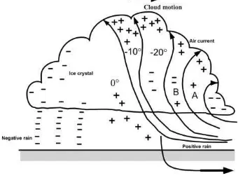
Lightning is a phenomenon that occurs when a charge accumulated in the clouds discharges to the ground, which is also a peak discharge [3]. Positive and negative charges become separated by the heavy air currents, with air crystals in the upper part and rain in the lower parts of the cloud during thunderstorms. Their charge probably centres at a distance of about 300 m to 2000 m while their charge separation is about 200 to 10,000 m, depending on the height of the cloud. Clouds have field gradients ranging from 100 V/cm to as high as 10 kV/cm at the initial discharge point and have potential of up to 107 to 108 V, while the energies that the cloud discharges are up to 250 kWh [3]. The upper regions of the cloud are usually positively charged, while the lower regions are negatively charged, but local regions within
the latter may be positive, as shown in Figure 1 [3].
Figure 1. Charge distribution with corresponding field gradient near the ground
There are three essential regions in the cloud according to Simpson’s theory, as shown in Figure 2. The air currents travel at above 800 cm/s and no raindrops fall below region A, while the air velocity is high enough to break the falling raindrops, which causes a positive charge spray in the cloud and a negative charge in the air in region A. The velocity decreases as the positively charged water drops recombine with the larger drops and this causes region A to be positively charged. Region B becomes negatively charged by the air currents and the temperature is low in the upper regions of the cloud [3].
Thunderclouds can also be defined as clouds in which lightning and sparks occur. Observations in many locations around the world state that a cumulonimbus cloud must Positively charged clouds move upwards and negatively charged clouds move downwards because of the polarization and then become thunderclouds. When a thundercloud grows and becomes unable to accumulate any more electricity, it will discharge to the ground.
Figure 3. Thundercloud process. (a) Generation of cloud (b) Thundercloud is formed by charging (c) Growth of
thundercloud (d) Lightning
Lightning is a transient, high-current electric discharge whose path length is measured in kilometres. Since the last century, many advanced instruments have been used to observe the electric and magnetic field data of lightning [4]. Lightning can move in cloud-to-ground, cloud-to-air, cloud-to-cloud, ground-to-cloud, and intra-cloud directions [1]. An isolated thundercloud can generate lightning at a few flashes per minute, while a severe storm can generate lightning at approximately ten flashes per minute and the maximum number of lightning flashes is about 85 in a minute.
Lightning activity is three times more frequent on land than over the ocean. The electric field generated by lightning flashes can be measured using an electric field mill, plate or whip antenna, whereas a crossed loop antenna is used to measure the magnetic field [5].
The current that flows from the electric field mill is given the background electric field can be obtained [5].
In investigations of electric fields using weather field instruments, the field in the clouds and the field gradients
were recorded at the earth’s surface [6].Changes in the
electric field strength and polarity were detected using a real-time monitor for the local thunder cloud and an early warning was sent when there was a change in the atmospheric electric field [7].
II. SOFTWARE DESIGN AND DEVELOPMENT
A. P r ogr a mme F lowcha r t for Collect Da ta a nd Rea d F ile
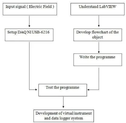
In this research, three stages will be implemented. The first stage is to develop a programme flowchart to collect data and a Read File data logger system. The next stage is to programme the virtual instrument using LabVIEW. The last stage is to test the data logger system. This is important to verify the result obtained from the simulation. The investigation consists of several phases to achieve the objective of the research. The first phase is the study of the physics of cloud profiles, followed by the visualization and simulation of cloud profiles using LabVIEW programming and the DAQ instrument. The last phase is result validation through a simulation using LabVIEW programming. The flowchart of the development of the research is shown in
Figure 5. Programme flowchart for collecting and saving data
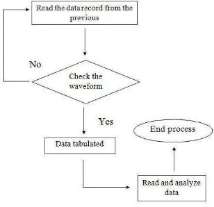
Figure 6. Program flowchart for reading data
In this project, LabVIEW programming was considered to be the most suitable software package compared to others in the market. LabVIEW is a very easy language for electrical or electronic engineers to pick up or learn, as the source code is very similar to circuit diagrams. Furthermore, LabVIEW also has raw speed for each development. The source code is written in a similar manner to many pre-defined components, i.e. drop-down and wired-in together menus.
The third advantage is LabVIEW’s compatibility with the National Instruments hardware when connected to their well-developed LabVIEW software.
B. Block Dia gr a m (La bVIEW)
The block diagrams were developed as shown in Figures 7, 8, 9 and 10. To develop the block diagrams, the function of each block component must be identified. In order to avoid error during the simulation, all pin inputs must be carefully placed. From the block diagram, the data was taken every second and it was saved every minute. The DAQ is used as an input and the waveform chart is displayed through the graph. This implementation is developed using LabVIEW and consists of three main groups: Input Block, Processing Block and Output Block. In Table 1, the details of these block components are explained. In this research, six inputs are used. All the block components were connected to form the required
input block diagram, as shown in Figure 7. The Input Block is used to generate the input signal.
TABLE 1. Simulation block components
No. Main Groups Block Components 1 Input Block DAQ Input, Sensors 1 to 6 2 Processing Block Write to measurement file
Amplitude and level measurement Simulate signal (DC)
Select signals Build table Create histogram Get Date / Time in second functions
Time interval
Build waveform (Analog waveform) function 3 Output Block Table
Select signal waveform chart All signals waveform chart Histograms 1 to 6
Figure 7. Block diagram for input block connection
Figure 8. Block diagram for processing block and output block connection
strength, while the y-axis describes the frequency distribution in terms of the frequency of the results [8].
The function of the amplitude and level measurements block is to make sure that all the signals are maintained in the DC signal and this enables computation of the signal
amplitude. This block was connected to the “build waveform” and “get date/data time in seconds function” block. The
function of the block component “get date/data time in seconds” is to make sure that the time in the programme is
equal to the laptop time. From there, the “write to measurement file” block is connected to save the data every
minute.
Lastly, the Processing Block is connected to the Output Block and is presented in the form of a graphical display. Then the tabulation of data is performed through the connection
with the “table” block component.
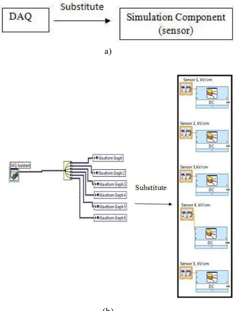
For simulation work, the DAQ is simulated using the simulation component (sensor). This is because there are 6 inputs and it is more appropriate to use a simulation component (sensor) rather than the DAQ and function generator. If the function generator and DAQ are to be used , the voltage must be divided and in parallel to get the right input voltage.
a)
(b)
Figure 9. (a) and (b) Substitution from DAQ assistant to simulation component
Figure 10 below presents the block diagram for the Read File. The Read From Measurement File is used to call back the previous data that have been saved and displayed in the form of a graphical and numeric display.
Figure 10. Block diagram for read file
III. RESULTS AND DISCUSSION
The data in Figure 11 is tabulated every second and saved every minute. The files are saved in a TDMS file and can only be called back using read file programming by LabVIEW. The programme is set to have a time interval of 100ms or 0.1s. All the sensors (Sensors 1 to 6) are set to run the programme. Figure 12 shows the “select signal” front panel, which can be selected as preferred by the user. The data is visualized using a waveform chart in terms of voltage (kV/cm) and time (s) in two different charts; all signals and select signal chart. The “all signals” waveform chart displays all the waveforms obtained, while the “select signal” waveform chart only displays the preferred signals.
Figure 13 shows the histogram of the data. The histogram obtained from the simulation shows the information where the x-axis represents the measurement scale of results for the ambient electric field strength and the y-axis describes the frequency of the electric field strength, showing how often the results occur. After all the data are saved, the data will be recalled using the Read File programme, as shown in Figure 14, and can be displayed.
Figure 12. Front panel of the waveform chart and “select signal”
Figure 13. Histogram of the data
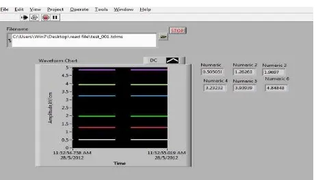
Figure 14. Read file as data logger
Several problems were encountered throughout the research. The main problem was caused by the inaccuracy of the data resulting from faulty equipment. During the experimental work, the pin from the DAQ, which was not secured tightly, could give a very bad connection and affect the results obtained. In addition, the over-sensitive DAQ system also influences the accuracy of results such as the detection of the electromagnetic field present in the surroundings. This was proven by the noise formation in the waveform, where the wave did not start at zero point. The data logger system will only show an accurate result when the waveform is started according to the user’s preferred set point. When the experiment was conducted, 3kV/cm was used to simulate the condition when lightning occurs. When lightning occurs at approximately 3kV/cm, the electric field strength is said to be very high at that point and it becomes
heavy. For this research, the data-reading format used is in a TDMS file and can only be opened using LabVIEW programming. Another front panel and block diagram were purposely created to easily read the previously obtained data. The front panel shows a waveform chart according to the data that has been saved every minute.
IV. CONCLUSION
The data logger system is used to manage the data obtained by the electronic components and the equipment used in the experiments. With the data being recorded carefully, the job of analysing and storing information on the magnitude of atmospheric electric field strength will be much easier and more accurate. The LabVIEW programme that has been developed will give a notification in the form of a waveform chart to show the condition of the atmospheric electric field strength.
ACKNOWLEDGEMENTS
The authors gratefully acknowledge the support extended by Ministry of Higher Education (MOHE), Malaysia and Universiti Teknologi Malaysia on the Fundamental Research Grant Scheme (FRGS), No. R.J130000.7823.4F054 to carry out this work.
REFERENCES
[1] Wendy L. Seaman, Captain, USAF (2000). Evolution of Cloud-To-Ground Lightning Discha rges in Tor na dic Thunder stor ms. Degree Thesis, Air Force Institute of Technology
[2] Katherine Miller, Alan Gadian, Clive Saunders, John Latham, and Hugh Christian (2001). Modelling and observations of thundercloud electrification and lightning. Atmospher ic Resea rch. 58(2001), 89-115 [3] M S Naidu, and V Kamaraju (2004). High Volta ge
Engineer ing. (3rd edition). Singapore: McGraw-Hill Education (Asia)
[4] Nianwen Xiang, and Shanqiang Gu (2011). A precisely synchronized platform for observing the lightning discharge processes. IEEE. 978(1), 1-4
[5] Vernon Cooray (2003). The Lightning F la sh. (1st edition). United Kingdom: The Institution of Electrical Engineers, London
[6] Edward Beck, Harold R. McNutt, Jr., Derrill F. Shankle, and Charles J. Tirk (1969). Electric fields in the vicinity of lightning strokes. IEEE Tr a ns on P ower Appa r a tus a nd Systems. 88(6), (904-910)