1-D DC Resistivity Inversion Using Singular Value Decomposition and Levenberg-Marquardt’s Inversion Schemes

(1)

Journal of Physics: Conference Series

PAPER • OPEN ACCESS

1-D DC Resistivity Inversion Using Singular Value

Decomposition and Levenberg-Marquardt’s

Inversion Schemes

To cite this article: M Heriyanto and W Srigutomo 2017 J. Phys.: Conf. Ser.877₀₁₂₀₆₆

View the article online for updates and enhancements.

1-D DC Resistivity Inversion Using Singular Value

Decomposition and Levenberg-Marquardt’s Inversion

Schemes

M Heriyanto and W Srigutomo

Physics of Earth and Complex System, Faculty of Mathematics and Natural Sciences, Institut Teknologi Bandung, Indonesia

mheriyanto37@gmail.com

Abstract. Exploration of natural or energy resources requires geophysical survey to determine the subsurface structure, such as DC resistivity method. In this research, field and synthetic data were used using Schlumberger configuration. One-dimensional (1-D) DC resistivity inversion was carried out using Singular Value Decomposition (SVD) and Levenberg-Marquardt (LM) techniques to obtain layered resistivity structure. We have developed software to perform both inversion methods accompanied by a user-friendly interface. Both of the methods were compared one another to determine the number of iteration, robust to noise, elapsed time of computation, and inversion results. SVD inversion generated faster process and better results than LM did. The inversion showed both of these methods were appropriate to interpret subsurface resistivity structure.

1. Introduction

DC Resistivity is one of geophysical exploration methods that can obtain subsurface resistivity structure. This method is frequently utilized for archeology surveys [15], mineral exploration [14], geothermal [13], and groundwater investigation [10,12].

Measurement principle of DC resistivity is injecting an amount of electric current into the earth to acquire potential difference on the surface thus apparent resistivity would be obtained based on Ohm’s law. Regarding its measurement configuration, this method is divided into some types, one of examples is Schlumberger configuration. This configuration is usually used for obtaining resistivity variation to its depth in 1-D orientation. Generally, resistivity model is interpreted in 2-D and 3-D domain, nevertheless for shallow structure and not too complex geology condition, interpretation can be done one-dimensionally. The apparent resistivity data acquired in the measurement is not real, thus interpretation demands an inversion process to obtain subsurface resistivity model. Several inversion methods which can be applied to apparent resistivity data in 1-D case are stable iterative [11], ridge regression [5]. Levenberg-Marquardt [3,9] and singular value decomposition [1] are methods that often be used for solving geophysical problem but there is still a few of scientists quantitatively comparing the advantages and disadvantages of these two methods.

(3)

1234567890

2. Forward Modeling and Inversion

Within this section, theories concerning forward modeling and inversion of DC resistivity with Schlumberger’s configuration are going to be explained.

2.1. Forward Modeling

As commonly used in forward modeling DC resistivity with Schlumberber’s configuration[1,4]. The

mathematical relation between Schlumberger’s apparent resistivity data and subsurface layer’s parameter can be described by Hankel’s integral.

( )

l l l l

formulation [7] as follows:

( )

(

)

where riand ti are resistivity and thickness of ith layer, NL is the consecutive number of layers. For

the last layer, TNL =rNL. Using fast Hankel transforms, that apparent resistivity data for DC resistivity

Schlumberger configuration can be calculated as [8]:

=

_å

( )

where Kis the number of coefficient and f_Kare the filter coefficients.

2.2. Inversion

Below is nonlinear relation between model parameter and data:

G

( )

m ₌d ₍₄₎

where d is vector of data with size of N x 1, G is nonlinear function relating data to model parameter

and m vector of model parameters with size of M x 1. N is number of data and M is number of models.

In this DC resistivity case, the data to be scrutinized is apparent resistivity (ra) vs AB/2 and the model

parameters are true resistivity (r) and layer’s thickness (t_).

Objective function to be minimized is [2]:

( )

å

( )

2.2.1. Levenberg-Marquardt Scheme. Iteration equation of model update in this method is expressed as follow [2,3]:

F is vector of differences between observed data and calculated data:

(4)

3 1234567890

where

Meanwhile, J(m) is a sensitivity matrix or Jacobi written as below:

( )

Thus equation (6) can be written as follow:

( ) ( )

Damping factor can be determined using golden section search (GSS) method [4] at each iteration.

2.2.2. Singular Value Decomposition Scheme. Iteration equation of model update in this method is

based on a formulation by Meju (1994), where matrix J to be factorized into 3 matrices:

T

USV

J₌ ₍₁₁₎

where U eigenvector of data with N x M size, V is eigenvector of model parameters with M x M size

and S is diagonal matrix containing non-zero eigenvalue of J as many as R with R ≤ M which R indicates

Rth iteration. Then equation (11) is substituted into equation (6) thus yields:

(

T

)

T

( )

k

Ekinci and Demirci (2008) has derived equation (13) and obtained solution equation for this inversion problem:

Damping factor is determined using formulation below [6]:

L

where L is test number performed and _Dx_{is formulated as follow:}

(5)

1234567890

3. Applications and Results

In this section both inversion methods were applied to synthetic and field data. In order to facilitate analyzing quantitatively, we employed parameter of data’s RMSE (root-mean-square error), models’ RMSE, number of iteration and elapsed computing time.

RMS error is defined as follow:

( )

where d is observed data and G

( )

_m _{is calculated data obtained from calculation of equation (4). Then}

relative RMSE is defined as data RMSE which is divided by d at each data and multiplied with 100%.

( )

m is the real model and the estimated model at ith iteration.

3.1. Synthetic data

LM and SVD methods were applied to inversion with 3 test models of homogenous earth (model 1), 3-layered (model 2), and noisy 3-3-layered (model 3).

Forward modeling data calculated from those 3 models were then inverted using LM and SVD. The result, those 3 sets of synthetic data obtained small RMS errors, it can be seen on table 2. This is also indicated by curve of apparent resistivity vs. AB/2 of which observed data and calculated data have fit figures to each other (see figure 1a), 1b), and 1c)).

Table 1. True and estimated models: (a) homogenous model; (b) noise-free model; (c) noisy model (15% random noise)

(6)

5 1234567890

Table 2. Observed and calculated apparent resistivity data of model 1 (a), model 2 (b), model 3 (c).

AB/2 (m)

Apparent resistivity (Ω m)

Model 1 Model 2 Model 3

Observed

Calculated

Observed

Calculated

Observed

Calculated

SVD LM SVD LM SVD LM

1 10 10 10 99.95 99.93 99.94 109.78 108.35 107.94

2 10 10 10 99.52 99.51 99.51 100.05 107.97 107.62

3 10 10 10 98.48 98.47 98.47 111.02 107.04 106.8

5 10 10 10 94.26 94.26 94.26 107.46 103.14 103.32

7 10 10 10 87.95 87.96 87.96 96.9 97 97.63

10 10 10 10 77.63 77.65 77.65 86.45 86.25 87.15

15 10 10 10 64.02 64.03 64.02 71.15 70.8 71.2

20 10 10 10 55.24 55.24 55.22 58.49 60.19 59.94

25 10 10 10 49.02 49.01 49 53.84 52.62 52.05

30 10 10 10 43.93 43.93 43.91 45.06 46.58 45.99

40 10 10 10 35.31 35.3 35.3 39.05 36.78 36.53

50 10 10 10 28.31 28.31 28.31 28.44 29.18 29.26

60 10 10 10 22.96 22.96 22.97 23.92 23.57 23.82

80 10 10 10 16.4 16.4 16.4 16.51 16.93 17.19

100 10 10 10 13.29 13.29 13.29 13.48 13.91 14.06

120 10 10 10 11.85 11.85 11.85 13.31 12.54 12.59

150 10 10 10 10.94 10.94 10.94 12.08 11.69 11.66

200 10 10 10 10.44 10.44 10.44 10.94 11.22 11.14

250 10 10 10 10.26 10.26 10.26 11.72 11.04 10.95

300 10 10 10 10.18 10.18 10.17 10.23 10.96 10.86

Data RMSE 1.8e-10 5.4e-15 0.0089 0.0097 2.389 2.369

Model RMSE 1.42 1.46 0.0089 0.014 1.785 1.613

Iter. No 94 11 57 87 100 100

Time (s) 59.19 11.63 36.7 84.23 14.22 95.19

The constructed homogenous model was a model with the same resistivity value over spaces and depth of 10 meters. Noisy 3-layered model, with random value of 15 % was constructed with 3 resistivity values and 2 layer’s thicknesses and final apparent resistivity multiplied by 15% random value of apparent resistivity.

Inversion result of those two methods depended on initial model. If the initial model was too far from solution model thus its inversion process would obtain big calculation data and model RMSE values, also get trapped in local minimum. In model 1, the initial model for inversion were three resistivity values of 5 Ω m and depth values of 5 m. Meanwhile in model 2 and 3, the initial model were 3 resistivity values of 80 Ω m with layer’s depth of 10 m.

(7)

1234567890

(8)

7 1234567890

Figure 1. Left curve presents observed and calculated apparent resistivity data using a) model 1 b) model 2 and c) model 3. Black dot, red triangle, and blue line show observed, SVD-inverted, and LM-inverted data respectively. Right curve presents subsurface model. Black line, red line, and blue line show true, SVD-inverted, and LM-inverted model respectively.

3.2. Field data

After examining LM and SVD using synthetic data, we implemented those methods to field data. We used Kaleköy’s data, located in northeastern part of Gökçeada [1]. Geological condition in the area has a thick sedimentary sequence, alluvium, and volcanic rock. The measurement was conducted using Iris Syscal-R1 + resistivity meter with maximum electrode space (AB) as long as 120 m.

Table 3. The estimated model of the field data

Model Parameter

Kaleköy Gobi, China

SVD LM SVD LM

ρ1 50.529 47.105 24.826 27.239

ρ2 18.862 10.665 69.653 77.219

ρ3 4.068 12.57 24.787 5.195

ρ4 219.527 388.252 474.424 343.836

t1 2.659 3.964 6.565 11.209

t2 10.577 38.927 38.886 64.411

t3 16.029 15.941 582.457 103.027

Data RMSE 0.686 1.6736 0.946 4.302

Iter. No. 100 100 100 100

(9)

1234567890

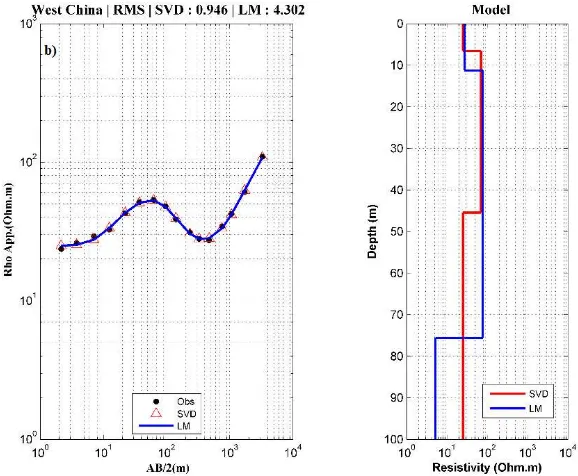
We selected the second field, Gobi area of West China [9]. Based on information provided by borehole measurement around the location, there were 4 layers of subsurface: Quaternary (0-4.63 m), Tertiary (4.63-48.34 m), Permian and Carboniferous (48.34-610 m), and Precambrian (basement).

The data inversion of both fields depended on initial model and model values would get trapped in

local minimum misfit if initial models was less good. We gave the initial models consisting of 4

resistivity models and 3 thickness models. Kaleköy’s inverted data had 0.686 and 1.6736 of data RMSE

(see table 3),meanwhile relative RMSE as much as 0.08% and 0.64% for SVD and LM respectively

while Gobi area’s had 0.946 and 4.302 of data RMSE (see table 3),meanwhilerelative RMSE as much

as 0.07% and 1.47% for SVD and LM respectively. Hence, it can be seen that SVD inversion obtained smaller data RMSE and relative RMSE than LM inversion did, which indicated the calculated data had a good fit with observed (field) data.

(10)

9 1234567890

Figure 2. Inversion result of a) Kaleköy’s data and b) Gobi area’s data, West China. Left curve presents observed and calculated apparent resistivity data. Black dot, red triangle, and blue line show observed data, calculated SVD, and calculated LM data respectively. Right curve presents subsurface model recovered values. Red and blue line indicate result using SVD and LM model respectively.

4. Discussion

Considering to synthetic data from test model in table 1, it can be seen that with the same initial model, LM inversion method was good to be used to invert synthetic data from model 1 (homogenous) and model 3 (3-layered noisy), while SVD inversion method was good to be used to invert synthetic data model 2 (3-layered noise-free). This was probably because of good GSS’s performance in determining damping factor when the constructed model was ideal (referred to synthetic data).

Computation time of LM inversion was longer than SVD inversion’s in spite of the same number of iteration. This was caused by selecting optimum damping factor value using GSS method as each LM inversion’s step must be evaluated within the range of damping factor value thus the inversion elapsed long computation time. Hence, it is recommended to use another method for determining the damping factor in order to make the inversion faster but still accurate in its results.

(11)

1234567890

5. Conclusions

We have successfully examined Levenberg-Marquardt and singular value decomposition inversion method, and compared them to each other. The LM method was good to be used in ideal synthetic data. However, we should better to use SVD in the field data case because this method is faster than LM and producing smaller number of iteration, relative RMSE and data RMSE than LM does.

Acknowledgments

The authors gratefully thank to Prihandhanu M. Pratomo for constructive comments and suggestions for improving the manuscript, Firman I. Bismillah for reviewing and editing the manuscript’s English structure, and all members of Modeling and Inversion Laboratory.

References

[1] Ekinci Y L and Demirci A 2008 A Damped Least-Squares Inversion Program for the

Interpretation of Schlumberger Sounding Curves J. of Appl. Sciences 8 (22): 4070-4078

[2] Srigutomo W, Agustine E, and Zen M H 2006 Quantitative Analysis of Self-Potential Anomaly:

Darivative Analysis, Least-Square Method and Non-Linier Inversion Indonesian Journal of

Physics17 No 2

[3] Rocky M and Srigutomo W 2015 Comparison of 1D Magnetotelluric Inversion using

Levenberg-Marquardt and Occam’s Inversion Schemes AIP Conf. Proc. 1656 070014-1-070014-4

[4] Vedanti N, Srivastava R P, Sagode J, and Dimri V P 2005 An efficient 1D OCCAM’S Inversion

Algorithm Using Analytically Computed First- and Second-order Derivatives for DC

Resistivity Sounding Computers & Geosciences31 319-328

[5] Meju M A 1992 An Effective Ridge Regression Procedure for Resistivity Data Inversion

Computers & Geosciences Vol 18 No 2/3 pp 99-118

[6] Arneson K and Hersir G P 1988 One Dimensional Inversion of Schlumberger Resistivity

Soundings: Computer Program, Description and User’s Guide: The United Nation University, Geothermal Training, Report 8, pp 59

[7] Koefoed O 1976 Error Propagation and Uncertainly in the Interpretation of Resistivity Data

Geophysical Prospecting24 31-48

[8] Ghosh D P 1971 Inverse Filter Coefficient for the Computation of Apparent Resistivity Standard

Curves for a Horizontally Layered Earth Geophysical Prospecting29 769-775

[9] Yin C 2000 Geoelectrical Inversion for One-dimensional Anisotropic Model and Inherent

Non-uniqueness Geophys. J. Int.140 11-23

[10] Harja A, Srigutomo W, Mustofa E J, and Sutarno D 2007 CSAMT and DC-Resistivity Survey for

Groundwater and Structural Investigation: Application to Eastern Bandung Basin, Indonesia

Proceesings of the 2007 Asian Physics Symposium ISBN 978-979-17090-1-9

[11] Jupp D L B and Vozoff 1974 Stable Iterative Methods for the Inversion of Geophysical Data

Gephys. J. R. Astr. Soc.42, 957-976

[12] Benson A K, Payne K L, and Stubben M A 1997 Mapping Groundwater Contamination using DC

Resistivity and VLF Geophysical Methods-a Case Study Geophysics62, 80-86

[13] Verave R T, Mosusu N, and Irarue P 2015 1D Interpretation of Schlumberger DC Resistivity Data

from the Talasea Geothermal Field West New Britain Province, Papua New Guinea

Proceedings World Geothermal Congress 2015

[14] Srigutomo W, Trimadona, Pratomo P M 2016 2D Resistivity and Induced Polarization

Measurement for Manganese Ore Exploration Journal of Physics: Conference Series 739,

012138

[15] Noel M and Xu B 1991 Archaeological Inverstigation by Electrical Resistivity Tomography: a

1-D DC Resistivity Inversion Using Singular Value Decomposition and Levenberg-Marquardt’s Inversion Schemes

Journal of Physics: Conference Series

1-D DC Resistivity Inversion Using Singular Value

Decomposition and Levenberg-Marquardt’s

Inversion Schemes

Related content

1-D DC Resistivity Inversion Using Singular Value

Decomposition and Levenberg-Marquardt’s Inversion

Schemes

( )

( )

( )

(

)

å

( )

( )

( )

å

( )

( )

( ) ( )

(

)

( )

( )

( )

( )

_å