Multimedia System
Digital Acquisition
ANALOG AND DIGITAL SIGNALS
● Analog signals are captured by a recording device, which attempts to
record a physical signal. A signal is analog if it can be represented by a continuous function.
● For instance, it might encode the changing amplitude with respect to an
input dimension(s).
● Digital signals, on the other hand, are represented by a discrete set of
values defined at specific (and most often regular) instances of the input domain, which might be time, space, or both.
● An example of a one-dimensional digital signal is shown in Figure 2-1,
where the analog signal is sensed at regular, fixed time intervals.
● Although the figure shows an example in one dimension (1D), the theory
The advantages of digital signals
over analog ones
● When media is represented digitally, it is possible to create complex, interactive content. ● Stored digital signals do not degrade over time or distance as analog signals do.
One of the most common artifacts of broadcast VHS video is ghosting, as stored VHS tapes lose their image quality by repeated usage and degradation of the medium over time. This is not the case with digital broadcasting or digitally stored media types.
● Digital data can be efficiently compressed and transmitted across digital networks.
This includes active and live distribution models, such as digital cable, video on demand, and passive distribution schemes, such as video on a DVD.
● It is easy to store digital data on magnetic media such as portable 3.5 inch, hard drives, or solid state
memory devices, such as flash drives, memory cards, and so on.
This is because the representation of digital data, whether audio, image, or video, is a set of binary values, regardless of data type. As such, digital data from any source can be stored on a common
ANALOG-TO-DIGITAL
CONVERSION
● The conversion of signals from analog to digital occurs via
two main processes: sampling and quantization.
● The reverse process of converting digital signals to analog
is known as interpolation.
● One of the most desirable properties in the analog to digital
conversion is to ensure that no artifacts are created in the digital data.
● That way, when the signal is converted back to the analog
Sampling
● Hence, Xs(1) = x(T); Xs(2) = X(2T ); Xs(3) = X(3T ); and so on.
● If you reduce T (increase f ), the number of samples increases; and correspondingly,
so does the storage requirement.
● Vice versa, if T increases (f decreases), the number of samples collected for the
signal decrease and so does the storage requirement.
● T is clearly a critical parameter. Should it be the same for every signal? If T is too
large, the signal might be under sampled, leading to artifacts, and if T is too small, the signal requires large amounts of storage, which might be redundant.
● For commonly used signals, sampling is done across one dimension (time, for sound
signals), two dimensions (spatial x and y, for images), or three dimensions (x, y, time for video, or x, y, z for sampling three-dimensional ranges).
● It is important to note that the sampling scheme described here is theoretical.
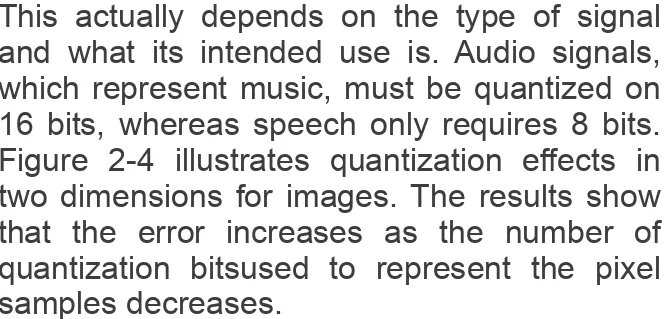
Quantization
● Quantization deals with encoding the signal value at
every sampled location with a predefined precision, defined by a number of levels.
● In other words, now that you have sampled a
continuous signal at specific regular time instances, how many bits do you use to represent the value of signal at each instance?
● Because each sample is represented by a finite number of
bits, the quantized value will differ from the actual signal value, thus always introducing an error.
● The maximum error is limited to half the quantization step.
● The error decreases as the number of bits used to
Bit Rate
● Understanding the digitization process from the previous
two subsections brings us to an important multimedia concept known as the bit rate, which describes the number of bits being produced per second.
● Bit rate is of critical importance when it comes to storing
a digital signal, or transmitting it across networks, which might have high, low, or even varying bandwidths.
● Bit rate, which is measured in terms of bits per second,
Signal
A signal is a set of data, usually a function of time. We denote a signal as x(t), where t is nominally time. We have already seen two types of signals:
● discrete signals, where t takes integer values, and
continuous signals, where t takes real values. In contrast, digital signals are those where the signal x(t) takes on
one of a quantized set of values, typically 0 and 1, and
● analog signals are those where the signal x(t) takes on
Type of Signal
● Continuous and smooth-such as a sinusoid
● Continuous and not smooth-such as a saw tooth
● Neither smooth nor continuous-for example, a step
edge
● Symetric-which can be further describe either as odd
(y=sin(x)) or even(y=cos(x))
● Finite support signals
● Periodic signal-a signal that repeats it self over a time
Linear Time Invariant System
● Any operation that transforms a signal is
called a system.
● Time invariance of a system can be defined by
Linear Time Invariant System
● Let a system transform an input signal x(t) into
Case For Linear System
Fundamental Result in Linear Time
Invariant System
Any LTI system is fully characterized by a specific function, which is called the impulse response of the system.
● The output of the system is the convolution of the input with the
system’s impulse response. This analysis is termed as the time domain point of view of the system.
● Alternatively, we can also express this result in the frequency
domain by defining the system’s transfer function. The transfer function is the Fourier transform of the system’s impulse
Convolution
The convolution of two signals f and g is
Convolution
● Compute the convolution of the functions x(t)
Case
● Solution: By convention, we assume that both
Fourier Transform
Transforms allow us to achieve three goals.
● The convolution of two functions, which arises in the computation
of the out- put of an LTI system, can be computed more easily by transforming the two functions, multiplying the transformed
functions, and then computing the inverse transform.
● Transforms convert a linear differential equation into a simpler
algebraic equation.
● They give insight into the natural response of a system: the
Useful functions in signal-processing theory: Delta function (top left), comb function (top right), step function (middle left), box
Sampling Theorem and Aliasing
● If these signals are to be digitized and
Sampling Theorem and Aliasing
The relationship states that the signal has to be sampled using a sampling frequency that is greater than twice the maximal frequency
This is an alternative statement of the Nyquist criterion and can be remembered as: To
What happens if your sampling frequency is higher than your Nyquist frequency? The
answer is: nothing special. When it comes to reproducing your analog signal, it is
guaranteed to have all the necessary
What happens if your sampling frequency is lower than your Nyquist frequency? In this case, you have a problem because all the
frequency content is not well captured during the digitization process. As a result, when the digital signal is heard/viewed or converted
Aliasing is the term used to describe loss of information during digitization. Such
undesirable effects are experi- enced for 1D signals such as sound, 2D signals such as
images and graphics, and even in 3D signals such as 3D graphics. Next, we discuss the
Aliasing
● Aliasing in Spatial Domains
Aliasing effects in the spatial domain are seen in all dimensions.
● Aliasing in the Temporal Domain
Examples of temporal aliasing can be seen in western movies, by observing the motion of stage coach wheels.
● Moiré Patterns and Aliasing
Another interesting example of aliasing, called the moiré effect, can occur when there is a pattern in the image being
Aliasing examples in the spatial domain. The top figure shows an example in one dimension, where original signal is shown along with sampled points and the reconstructed signal. The bottom set of figures show a 2D input image signal. The top left
shows the original signal and the remaining three show examples of the signal reconstruction at different sampling resolutions. In all cases, the output does not match
Moiré pattern example. The vertical bar pattern shown on the top left is
rotated at an angle to form the input signal for sampling. The bottom row illustrates the sampling process. A sampling grid is superimposed to produce a sampled output.
The grid resolution corresponds to the sampling resolution. The middle figure in the second row shows the sampled values at the grid locations and the right figure
Filtering
● The sampling theorem states sampling requirements
to correctly convert an analog signal to a digital signal.
● Input analog frequency range can enable this
conversion
● Analog filtering techniques are commonly used to
capture a variety of commonly used signals such as audio and images. However, in the digital world,
Digital Filters
● In signal processing, the function of a filter is to
remove unwanted parts of the signal, such as
random noise and undesired frequencies, and to extract useful parts of the signal.
● There are two main kinds of filters: analog and
digital.
● Analog filter uses analog electronic circuits made up
Advantages of Digital Filters
● A digital filter is programmable
● Digital filters are easily designed, tested, and implemented on a
general-purpose computer or workstation
● Digital filters can be combined in parallel or cascaded in series with
relative ease by imposing minimal software requirements.
● The characteristics of analog filter circuits (particularly those
containing active components) are subject to drift and are dependent on temperature.
● Unlike their analog counterparts, digital filters can handle
Filtering Dimension
● Filtering in 1D
A 1D signal is normally represented in the time domain with the x-axis showing sampled positions and the y-axis
showing the amplitude values.
● Filtering in 2D
Digital filtering on images—The top row depicts an image and its frequency transform, showing frequencies in two dimensions. The middle row shows the effect of a low-pass filter. Here, only the frequencies inside
Subsampling
● Filtering data prior to sampling is, thus, a practical
solution to acquiring the necessary quantity of reliable digitized data. The cut off frequency of the filter
depends largely on the signal being digitized and its intended usage. However, once in the digital domain, there is frequently a need to further decrease (or