1. Study Program of Oceanography, GM-ITB
Catatan : Usulan makalah dikirimkan pada Juli 2005 dan dinilai oleh peer reviewer pada tanggal 02 Agustus 2005 - 14
Nopember 2005. Revisi penulisan dilakukan antara tanggal 18 Nopember hingga 19 Januari 2006. Abstract
A coupled three-dimensional hydrodynamics and sediment transport model of HydroQual, Inc., (2002), ECOMSED, has been used to simulate variation of suspended cohesive sediment transport in Estuary of Mahakam Delta. The simulation results indicate that tides and seasonal variation of river discharges are the main causes of variations in the suspended sediment concentration in this area.
A one-year simulation of suspended sediment distribution shows that the suspended cohesive sediment discharge to the Makassar Strait is mainly transported southward, namely through locations of Muara Jawa and Muara Pegah and seems to reach a maximum distance of distribution in January and a minimum one in October. The simulation results also show that river discharges less influence the suspended sediment concentration at Tanjung Bayur, which is located at the tip of the channel in the middle, compared to the other locations.
Keywords: Three-dimensional hydrodynamics and sediment transport models, Estuary of Mahakam Delta,
Suspended cohesive sediment concentration, Tides, River discharges.
Abstrak
Suatu model kopel tiga dimensi hidrodinamika dan transpor sedimen HydroQual, Inc., (2002), ECOMSED, diterapkan untuk mensimulasi variasi transpor sedimen kohesif melayang di Estuari Delta Mahakam. Hasil simulasi menunjukkan bahwa pasut dan variasi musiman dari debit sungai adalah penyebab utama dari variasi konsentrasi sedimen melayang di daerah ini.
Simulasi satu tahun distribusi sedimen melayang memperlihatkan bahwa sedimen kohesif yang memasuki Selat Makassar terutama ditransporkan ke arah selatan melalui Muara Jawa dan Muara Pegah.
Jangkauan maksimum dari aliran sedimen memasuki Selat Makassar terjadi pada bulan Januari dan minimum pada bulan Oktober. Hasil simulasi juga menunjukkan bahwa pengaruh debit sungai terhadap konsentrasi sedimen di Tanjung Bayur lebih kecil daripada di lokasi-lokasi yang lain.
Kata-kata kunci: Model hidrodinamika dan transpor sedimen tiga dimensi, Estuuri Delta Mahakam,
konsentrasi sedimen kohesif melayang, pasut, debit sungai.
Study on Seasonal Variation of Cohesive Suspended Sediment Transport
in Estuary of Mahakam Delta
by using A Numerical Model
Safwan Hadi1)
Nining Sari Ningsih1)
Ayi Tarya1)
TEKNIK
SIPIL
1. Introduction
Estuaries are transitional areas that trap abundance of particulate and dissolved matter that come from various sources. Estuaries play an important role in filtering sediment that goes to the sea. This filtering role makes them crucial systems for study the effect of human activities to sediment dynamics which in the long run will affect morphological evolution of the estuaries, such as migration of river mouth and
formation of deltas. In estuaries tides and tidal current are two major driving forces, which play important roles in transporting sediment and shaping their morphologies.
activities of human beings, such as living marine resource in the form of fish and shellfish, transportation, and recreation. In addition, the coastal area of Mahakam Estuary, which has high primary productivity, is potential for developing aquaculture farming, especially shrimps and fishes. Fishing industry (e.g., shrimp pond culture) has been rapidly developed in the area.
Unfortunately, the harmful effects of society on this resource such as marine pollution, poor control of aquatic environment and of fisheries management, and also poor understanding of transport processes of sediments in suspension have resulted in documented cases of reduced yields in some of the major commercial fisheries and deposition in waterways which requires high cost of dredging. Influence of sediments in the estuary is not only limited to its role on material transport and deposition but also to the estuarine ecosystem.
The suspended sediments play an important role in an estuary because they provide habitat for benthic organism, transport absorbed toxic substances, and limit light availability. Dense cohesive sediment suspensions could inhibit light penetration, affect photosynthesis and causing a decrease in phytoplankton production, and consequently affect the whole food chain.
To overcome this problem, an understanding of relationships between the physical environment and marine ecosystem is required. In general, optimal conditions of temperature, salinity, and circulation will produce abundant fish stocks, whereas unfavorable environmental conditions can lower abundance. Therefore, both for scientific and practical reasons it is desirable to have a better understanding on the management of living marine resources and to have the ability to predict accurately the sediment transport processes in the estuary.
The Mahakam Estuary provides an ideal case for studying estuarine dynamic and sediment transport. For centuries sediments have been carried by Mahakam River and trapped in the Mahakam Estuary to form Mahakam Deltas. Interaction between fresh water flow and tides and tidal current entering from strait of Makassar plays an important role in forming the deltas.
With the development of both computer and numerical methods by means of mathematical equations for solutions of time-dependent flows, numerical simulation has become an economic and effective way to obtain the required flow parameters and to provide a gain insight to sediment transport processes compared to the high cost of performing field observations. Mathematical modelling has been
extensively applied in sedimentary studies in estuaries. It gives significant contribution for understanding and prediction of estuarine problems that allows developing a rational contingency planning.
Therefore, in this paper we address to model water circulation pattern and suspended sediment transport in the Mahakam Estuary by using a fully integrated three-dimensional (3D) hydrodynamic and sediment transport model, ECOMSED, developed by HydroQual, Inc., (2002), USA.
2. Methodology
Simulation of suspended sediment in the Mahakam Estuary was carried out by means of the coupled 3D hydrodynamics and sediment transport model. The 3D hydrodynamics model was used to simulate water circulation in the area and to generate current field as the input for sediment transport model. The sediment transport model was then run to simulate the movement of suspended cohesive sediment in the area.
2.1 Hydrodynamic model
The hydrodynamic model is described by the conservation laws of momentum and water mass which is represented by the following governing equations:
The continuity equation is:
The momentum equations are:
where U, V, and W are velocity
components in x, y, and z direction
respectively; t is time; ροis the reference density; ρ is
the in situ density; g is the gravitational acceleration; P
is the pressure; KM is the vertical eddy diffusivity of
turbulent momentum mixing; f is the Coriolis
parameter; and Fx and Fy represent the terms of
horizontal mixing processes.
2.2 Sediment transport model
The sediment transport model used in this study is the 3D advection-dispersion equation for transport of sediment, as follow:
where C represents the concentration of suspended
sediment; Ws is the suspended sediment settling
velocity; t is time, and U, V, W are velocity in x, y, and
z direction respectively; AH is horizontal diffusivity;
and KH = vertical eddy diffusivity.
In solving the governing Equation (5), boundary
conditions needed to be prescribed, as follow:
where E and D are resuspension and deposition flux
respectively; η = water surface elevation; and H =
bathymetric depth.
2.2.1 Deposition of cohesive sediments
The deposition rate for cohesive sediments depends directly upon the sediment flux approaching the bed and the probability of the flocs sticking to the bed and is commonly described by the formula presented by Krone (1962) as follow:
in which D is depositional flux; Ws is settling velocity
of the cohesive sediment flocs; C is cohesive
suspended sediment concentration near the
sediment-water interface; and P = probability of deposition.
2.2.2 Resuspension of cohesive sediments
Based on both laboratory experiments (Parchure and
Mehta, 1985; Tsai and Lick, 1987; Graham, et al.,
1992) and field studies (Hawley, 1991; Amos et al.,
1992), it has been reported that only a finite amount of sediment can be resuspended from a cohesive sediment bed exposed to a constant shear stress as a result of armoring. According to formulation of
Gailani et al. (1991), the amount of fine-grained
sediment resuspended from a cohesive sediment bed can be written as:
where ε is resuspension potential; a0 is constant
depending upon the bed properties; Td is time after
deposition; τb is bed shear stress; τc is critical shear
stress for erosion; and m, n = constants dependent
upon the depositional environment.
The resuspension rate of sediments, which is needed in
the Equation (6b), is then given by
where f is fraction of sediment in cohesive bed and .
3. Model Application
3.1 Model area
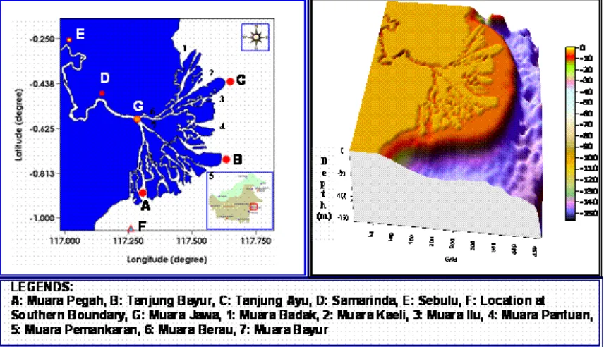
Figure 1 shows the computational domain and
bathymetry of Mahakam Estuary located at 0o 10' 00" -
1o 03' 00" S and 116o 59' 00" - 118o 00' 00" E. The model area comprises Mahakam River, Delta of Mahakam and western part of Makassar Strait. The region of Mahakam Estuary was simulated in the model using horizontally finite difference mesh of 468 x 490 grid squares, equally spaced at 200 m interval,
and vertical grid of 3 σ-levels (Figure 1).
3.2 Simulation design
The main forcing for the model is tidal elevation, which is imposed at the open sea boundaries and is obtained by carrying out tidal prediction based on 8 tidal constituents (M2, S2, N2, K2, K1, O1, P1, and Q1) published by the Ocean Research Institute, University of Tokyo. In addition to the tidal elevation data, initial data of temperature, salinity, and suspended sediment concentration were supplied to the model in order to realistically compute water circulation, temperature, salinity, and transport of sediments. The initial temperature and salinity data were taken from the Levitus data (1982) and the Indonesian Institute of Sciences, whereas the initial data of suspended sediment concentration were supplied by the Indonesian Institute of Sciences.
Allen et al (1979) in Davis (1985) have reported that
water circulation pattern in Estuary of Mahakam Delta is dominantly affected by tides and since the area is incised by fluvial distributaries (river channels) and tidal channels, which are relatively narrow, wind effect on water circulation in the area is neglected in the present study. Hence, in responses to seasonal changes of the monsoon mechanism, which generally plays an important role in the Indonesian coastal ocean circulation, mean monthly discharge of the Mahakam River, in which showing large seasonal variation, was
taken as the model input (Figure 2).
A one-year simulation of river discharge-and tide-driven circulation in 2005 was then carried out to
Figure 1. Computational domain and bathymetry of Mahakam Estuary (Source: Dishidros TNI AL, 2003)
obtain a better understanding of suspended sediment distribution of turbid coastal water of the Mahakam Delta and to investigate its variability.
4. Results and Discussions
4.1. Model verification
4.1.1 Hydrodynamic model
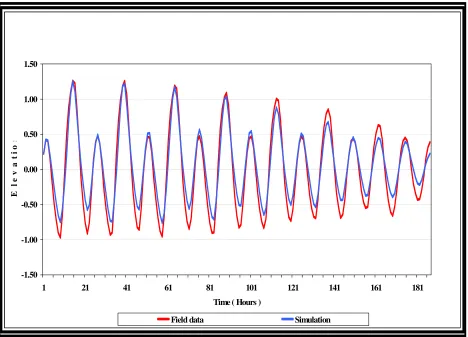
For model verification, the simulated water surface elevation is compared to that of field measurements at
Muara Jawa (marked G in Figure 1), which is carried
out by Tuijnder (2003) from IMAU (Institute for
Marine and Atmospheric Research Utrecht), Utrecht
University, the Netherlands. The verification results of
water elevation at that place can be seen in Figure 3.
From the figure, it is shown that the model predicts the free surface elevation quite well, mainly for the tidal phases, but the amplitude smaller in the order of less than 0.3 m.
Current velocities are complement of the tidal
elevation. Figure 4(a) shows comparison of the
predicted and measured surface velocity component in
x direction (U) of Tuijnder (2003) in the period of 30
June - 8 July 2003 at Muara Jawa (marked G in Figure
1). Generally, one can see that the simulated surface
velocity shows a good agreement with that of the measured one, mainly for the tidal current phases. However, the magnitude of predicted results is weaker, with a mean error of about 39.73 %. The difference between the predicted and measured results is probably caused by the estimation of the effect of the bottom friction which does not reproduce adequately
the nonlinear interaction of the extremely strong tidal currents with the bottom topography. In addition, the inaccurate discharge rate from surrounding rivers may also contribute to the error of prediction.
4.1.2 Sediment transport model
In this study, the simulated suspended concentration of cohesive sediment is compared to that of field
measurements at Muara Jawa (marked G in Figure 1)
carried out by Tuijnder (2003) and is also compared to the field data of Budhiman (2004).
Figure 4(b) shows comparison of the predicted and
measured suspended concentration of Tuijnder (2003) in the period of 30 June - 8 July 2003 at Muara Jawa
(marked G in Figure 1, at depth of about 4 m). As can
be seen, model results agree well with the general trend of the measured data. In general, the agreement between the numerically simulated and the measured concentration is reasonably encouraging, with a mean error of about 38.74 %. The difference between the model results and the field data is probably due to the inaccurate definition of the sediment source from the Mahakam River. The inaccurate discharge rate of the suspended sediment from the river and the assumption of homogenous cohesive sediment in the computational domain can be other sources of inaccurate prediction.
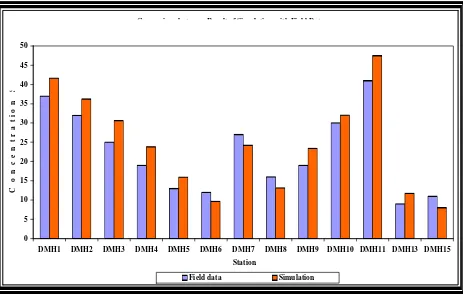
Meanwhile, the comparison of suspended sediment concentration between the predicted and the measured results of Budhiman (2004) in the period of 3 - 5 July
R i v e r D i s c h a r g e s M e a n M o n t h l y K o t a B a n g u n S a m a r i n d a Y e a r 1 9 9 3 - 1 9 9 8 .
Figure 2. Mean monthly discharge of the Mahakam River based on data of 1993-1998
(Source: Research Institute for Water Resource Development, the Ministry of Public Works, Indonesia, 2003)
see, from the Figure 5, the simulation results show a
good agreement with the measured data, with a mean error of about 19.05 %.
4.2 Simulation results
4.2.1 Surface water circulation pattern
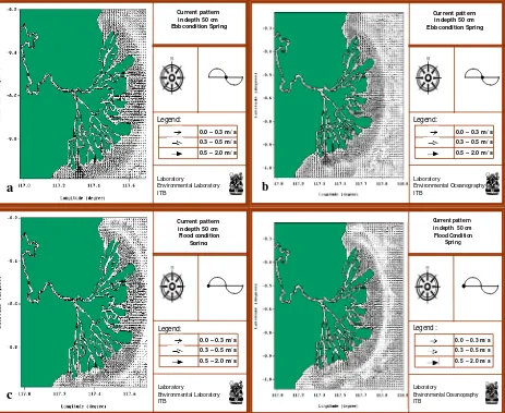
Figure 6 shows tide- and river discharge-driven
circulation at depth of 0.5 m for spring ebb and flood condition in January and October, respectively. Tidal
elevation at Muara Jawa (marked G in Figure 1) was
chosen as the reference time of the flood and ebb condition. The figure clearly shows the existence of currents that flow back and forth representing flood
and ebb conditions. At spring ebb condition (Figures
6a and 6b), the currents coming from the Mahakam
River flow into the Makassar Strait through river and tidal channels that exist in the Estuary of Mahakam
Delta. Otherwise, at spring flood condition (Figures
6c and 6d) they flow into the Mahakam River. The
river discharges clearly influence the circulation. The river discharge in January is stronger than that in October. Consequently, one can observe that at spring ebb condition there is an increase of the magnitude of the currents in January compared to that in October
(Figures 6a and 6b). In addition, it is found that the
currents coming from the Mahakam River flow into the Makassar Strait mainly through Muara Pegah
(marked A in Figure 1).
4.2.2 Sediment concentration distribution pattern
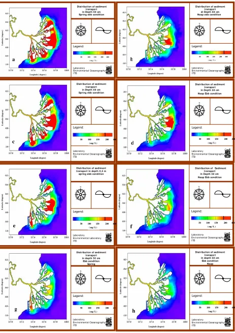
Figure 7 shows distribution of predicted sediment
concentration at depth of 0.5 m in January (7a and
7b), in April (7c and 7d), in July (7e and 7f), and in
October (7g and 7h) for spring and neap ebb
condition, respectively.
From the Figure 7, one can see that the suspended
cohesive sediment discharged to the Makassar Strait from the Mahakam River is mainly transported southward, namely through the Muara Jawa and the
Muara Pegah (marked G and A in Figure 1,
respectively).
The one-year simulation of suspended sediment distribution shows that the sediments seems to spread farthest in February and reach minimum distance of distribution in October in accordance with the monthly sediment discharge of the Mahakam River.
The magnitude of the currents during spring tide is stronger that that during the neap one and as a consequence it results in the greatest bed erosion. Hence, the suspended sediment concentration during spring tide is higher that that during the neap one.
4.2.3 Correlation between the river discharges and the suspended sediment concentration
Figure 8a shows correlation between the Mahakam
River discharges and the suspended sediment concentration (SSC) at Muara Pegah (marked A in
Figure 1) for spring ebb condition. Meanwhile,
Figure 8b shows correlation values between the
Mahakam River discharges and the SSC at Muara Pegah, Muara Jawa, Muara Pantuan, Muara Kaeli, and
Tanjung Bayur (marked G, A, 4, 2, and B in Figure 1,
respectively) for spring and neap tides.
From the figures, one can see that there is a strong correlation between the Mahakam River discharges and the SSC, namely the stronger river discharges exist, the higher SSC will occur. The correlation values between the Mahakam River discharges and the
SSC at Tanjung Bayur (marked B in Figure 1) are
smaller than those at the other regions (Figure 8b).
strong tidal current is more dominant to cause the high SSC compared to the suspended sediment discharges from the Mahakam River.
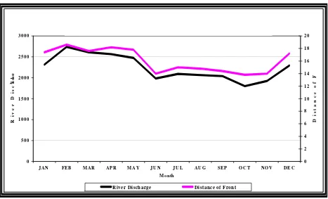
4.2.4 Correlation between the river discharges and distances of turbidity front
Correlation between the Mahakam river discharges and distances of turbidity front from Muara Pegah
(marked A in Figure 1) towards the Makassar Strait
for neap ebb condition can be seen in Figure 9. In this
study, the SSC of about 150 mg/l was chosen as the reference value to determine the turbidity front. From
the Figure 9, it is found that at the region there is a
strong correlation between the Mahakam River discharges and the distance of the turbidity front, namely the stronger river discharges exist, the farther distance of turbidity front will be.
The simulation results in Figure 9 show that the
maximum distance of the turbidity front of about 18.6 km occurs in February, while the minimum one of about 13.2 km occurs in October. The correlation values between the Mahakam River discharges and the distances of the turbidity front from the Muara Pegah
(marked A in Figure 1) are r =0.74 (for spring ebb
condition ), r = 0.96 (for neap ebb condition ), r = 0.22 (for spring flood condition), and r = 0.76 (for neap flood condition). As can be seen from the calculated correlation values, the ebb conditions are more dominant on increasing the distance of the turbidity front because the river discharge-driven currents flow in the same direction to the tide-driven circulation during the ebb conditions.
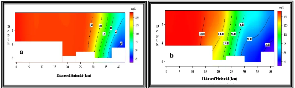
To obtain a better understanding of the variation of turbidity front distances from Muara Jawa to Muara
Pegah (marked G – A in Figure 1, respectively), we
made the vertical profile of suspended sediment concentration. Figures 10a and 10b show distribution of the suspended sediment concentration in transect along the Muara Jawa – Muara Pegah during neap ebb condition in January and in October, respectively. The
simulation results in Figures 10a and 10b show that
the high suspended sediment concentration is increasing with distance from Muara Jawa to Muara Pegah in February than that in October. In this condition, the maximum distance of the turbidity front of about 30 km occurs in February, while the minimum one of about 17 km occurs in October. Verification of Elevation result Simulation With Field Data in Estuary of Jawa
-1.50 -1.00 -0.50 0.00 0.50 1.00 1.50
1 21 41 61 81 101 121 141 161 181
Time ( Hours )
El
e
v
a
t
i
o
n
Field data Simulation
Figure 3. Sea level comparison between the simulation results and field data of IMAU in the period of 30 June 2003 to 8 July 2003 at Muara Jawa
Verification Component Velocity of U in Estuary of Jawa ( June 30 - July 8, 2003 )
-0.2 -0.15 -0.1 -0.05 0 0.05 0.1 0.15 0.2
1 21 41 61 81 101 121 141 161 181
Time ( Hours )
Ve
lo
ci
ty
(
m
/s
)
Simulation Field data
Verification of Concentration Sediment in Estuary Java Depth 4 m ( June 30 - July 8, 2003 )
0 50 100 150 200 250 300
1 21 41 61 81 101 121 141 161 181
Time ( Hours )
Conc
en
tr
ation Se
dim
en
t
( m
g
/L
Field data Simulation
(a)
(b)
Figure 4. Model verification of (a) velocity components in x direction (U); (b) suspended sediment concentration at depth of about 4 m between the simulation results and field data of IMAU in
the period of 30 June 2003 to 8 July 2003 at Muara Jawa (marked G in Figure 1).
Comparison between Result of Simulation with Field Data 3 - 5 July 2003.
0 5 10 15 20 25 30 35 40 45 50
DMH1 DMH2 DMH3 DMH4 DMH5 DMH6 DMH7 DMH8 DMH9 DMH10 DMH11 DMH13 DMH15
Station
C
o
n
cen
t
ra
t
i
o
n
S
Field data Simulation
Current pattern in depth 50 cm Ebb condition Spring
Legend:
Laboratory Environmental Laboratory ITB
0.0 – 0.3 m/ s 0.3 – 0.5 m/ s 0.5 – 2.0 m/ s
Current pattern in depth 50 cm Ebb condition Spring
Legend:
Laboratory
Environmental Oceanography ITB
0.0 – 0.3 m/ s 0.3 – 0.5 m/ s 0.5 – 2.0 m/ s
a
bCurrent pattern in depth 50 cm Flood condition
Spring
Legend:
Laboratory Environmental Laboratory ITB
0.0 – 0.3 m/ s 0.3 – 0.5 m/ s 0.5 – 2.0 m/ s
c
d
Current pattern in depth 50 cm Flood Condition
Spring
Legend:
Laboratory
Environmental Oceanography ITB
0.0 – 0.3 m/ s 0.3 – 0.5 m/ s 0.5 – 2.0 m/ s
Dist ribut ion of Sediment transport in Depth 5 0 cm
Neap Ebb condit ion
Legend:
Dist ribut ionof sediment transport
Dist ribut ion of sediment transport
Dist ribut ion of sediment transport in Depth 5 0 cm Neap Ebb condit ion
Legend:
Dist ribut ionof sediment transport
Dist ribut ion of sediment transport inDepth 5 0 cm Spring ebb condit ion
Legend:
Dist ribut ion of sediment
e
Dist ribut ion of sediment transport in depth 0,5 m spring ebb condition
Figure 7. Predicted sediment concentration distribution at depth of 0.,5 m in January (a and b), in April (c and d), in July (e and f), and in October (g and h) for spring and neap ebb
Overlay between river discharge and sediment concentration in Muara Pegah
Jan Feb Mar Apr May Jun Jul Aug Sep Oct Nov Dec
Ri
Sediment Concentration River Discharge
Correlation between river discharge of Mahakam with concentration sediment
0.84
Estuary of Pegah Estuary of Jawa Estuary of Pantuan Estuary of Kaeli Cape of Bayur Estuary
Figure 8. (a). Correlation between the Mahakam River discharges and the suspended sediment concentration (SSC) at Muara Pegah (marked A in Figure 1) for spring ebb condition; (b). Correlation values
between the Mahakam River discharges and the SSC at Muara Pegah, Muara Jawa, Muara Pantuan, Muara Kaeli, and Tanjung Bayur (marked G, A, 4, 2, and B, respectively) for spring and neap tides
C om p arison o f D istan ce F ron t of E stu a ry of P eg ah w ith R ive r D isch ar ge o f M ah a k am
Distance of Horizontal ( km ) D
e p t h
Distance of Horizontal ( km ) D
Figure 10. Suspended sediment concentration in transect along Muara Jawa – Muara Pegah (marked G – A in Figure 1) at neap ebb condition; (a).in January, (b). in October.
5. Conclusions
The coupled 3D hydrodynamics and sediment transport model called ECOMSED has been applied to predict suspended cohesive sediment fluxes in the Estuary of Mahakam Delta whose environment has been rapidly changing due to the development of its coastal area, such as development of extensive aquaculture (shrimp ponds), deforestation upstream locations, and conversion of mangrove forest. This causes many hazardous situations such as catastrophic beach erosion and disrupted navigation because of the excess of sediment materials.
The application of the model to the Mahakam Estuary showed that tides and seasonal variation of river discharges are the main causes of variations in the SSC in this area. At spring tide, the SSC is higher that that during the neap one due to the stronger current. Meanwhile, during the neap tide, river channels of this region have higher SSC because of the ebb current and river discharge.
The one-year simulation of suspended sediment distribution shows that the suspended cohesive sediment is mainly transported southward, namely through the Muara Jawa and the Muara Pegah (marked
G and A in Figure 1, respectively) and seems to
spread farthest in February and reach minimum distance of distribution in October. The investigation of correlation between the river discharges and the SSC at some areas shows that the river discharge less influences the SSC at Tanjung Bayur (marked B in
Figure 1) compared to the other locations.
In general, the coupled 3D hydrodynamics and sediment transport model used in this study is able to simulate suspended sediment transport in the Mahakam delta waters. The application of the model to the area can also be extended to predict the morphological processes, namely bed level changes and beach erosion. As an extension of this research program, these kinds of studies are currently being conducted.
6. Acknowledgements
We gratefully acknowledge the support from the Ministry of Research and Technology of Republic of Indonesia for funding this research under grants of RUT-XI.
References
Amos, C. L., Grant, J., Daborn, G. R., and Black, K.,
1992, “Sea Carousel – A Benthic, Annular
Flume”, Estuar. Coast. And Shelf Sci.,
34:557-577.
Budhiman, S., 2004, “Mapping TSM Concentrations
from Multisensor Satellite Images in Turbid Tropical Coastal Waters of Mahakam Delta,
Indonesia”, Master of Science Thesis, ITC,
Enschede, The Netherlands.
Davis, R. A., (eds.), 1985, “Coastal Sedimentary
Environments”, Springer-Verlag New York Inc.
Gailani, J., Ziegler, C. K., and Lick, W., 1991,
“The Transport of Sediments in the Fox River”,
J. Great Lakes Res., 17: 479-494.
Graham, D. I., James, P.W., Jones, T. E. R., Davies, J.
M., and Delo, E. A., 1992, “Measurement and
Prediction of Surface Shear Stress in Annular
Flume”, ASCE J. Hydr. Engr.,
118(9):1270-1286.
Hawley, N., 1991, “Preliminary Observations of
Sediment Erosion from a Bottom Resting
Flume”, J. Great Lakes Res., 17(3):361-367.
HydroQual, Inc., 2002, “A primer for ECOMSED”,
Users Manual, Mahwah, N. J. 07430, USA.
Krone, R. B., 1962, “Flume studies of the transport of
sediment in estuarial processes”, Final Report,
Levitus, S., 1982, “Climatological Atlas of the World
Ocean”, U.S. Department of Commerce,
National Oceanographic and Atmospheric
Administration, Tech. Rep. 13: 173 pp.
Parchure, T. M., and Mehta, A. J., 1985, “Erosion of
Soft Cohesive Sediment Deposits”, ASCE J.
Hydr. Engr., 111(10):1308-1326.
Tsai, C. H., and Lick, W., 1987, “Resuspension of
sediments from Long Island Sound”, Wat. Sci.
Tech., 21(6/7):155-184.
Tuijnder, A., 2003, “Estimation of spatial scales of
mixing processes of freshwater and seawater in the Berau River Delta and Mahakam River
Delta, East Kalimantan”, Department of