About the authors
Professor R. E. Smallman
After gaining his PhD in 1953, Professor Smallman spent five years at the Atomic Energy Research Estab-lishment at Harwell, before returning to the University of Birmingham where he became Professor of Physi-cal Metallurgy in 1964 and Feeney Professor and Head of the Department of Physical Metallurgy and Science of Materials in 1969. He subsequently became Head of the amalgamated Department of Metallurgy and Materials (1981), Dean of the Faculty of Science and Engineering, and the first Dean of the newly-created Engineering Faculty in 1985. For five years he was Vice-Principal of the University (1987–92).
He has held visiting professorship appointments at the University of Stanford, Berkeley, Pennsylvania (USA), New South Wales (Australia), Hong Kong and Cape Town and has received Honorary Doctorates from the University of Novi Sad (Yugoslavia) and the University of Wales. His research work has been recognized by the award of the Sir George Beilby Gold Medal of the Royal Institute of Chemistry and Institute of Metals (1969), the Rosenhain Medal of the Institute of Metals for contributions to Physical Metallurgy (1972) and the Platinum Medal, the premier medal of the Institute of Materials (1989).
He was elected a Fellow of the Royal Society (1986), a Fellow of the Royal Academy of Engineer-ing (1990) and appointed a Commander of the British Empire (CBE) in 1992. A former Council Member of the Science and Engineering Research Council, he has
been Vice President of the Institute of Materials and President of the Federated European Materials Soci-eties. Since retirement he has been academic consultant for a number of institutions both in the UK and over-seas.
R. J. Bishop
Modern Physical Metallurgy
and Materials Engineering
Science, process, applications
Sixth Edition
R. E. Smallman,
CBE, DSc, FRS, FREng, FIM
R. J. Bishop,
PhD, CEng, MIM
Butterworth-Heinemann
Linacre House, Jordan Hill, Oxford OX2 8DP 225 Wildwood Avenue, Woburn, MA 01801-2041
A division of Reed Educational and Professional Publishing Ltd
First published 1962 Second edition 1963 Reprinted 1965, 1968 Third edition 1970
Reprinted 1976 (twice), 1980, 1983 Fourth edition 1985
Reprinted 1990, 1992 Fifth edition 1995 Sixth edition 1999
Reed Educational and Professional Publishing Ltd 1995, 1999
All rights reserved. No part of this publication may be reproduced in any material form (including photocopy-ing or storphotocopy-ing in any medium by electronic means and whether or not transiently or incidentally to some other use of this publication) without the written permission of the copyright holder except in accordance with the provisions of the Copyright, Designs and Patents Act 1988 or under the terms of a licence issued by the Copyright Licensing Agency Ltd, 90 Tottenham Court Road, London, England W1P 9HE. Applications for the copyright holder’s written permission to reproduce any part of this publication should be addressed to the publishers
British Library Cataloguing in Publication Data
A catalogue record for this book is available from the British Library
Library of Congress Cataloguing in Publication Data
A catalogue record for this book is available from the Library of Congress
ISBN 0 7506 4564 4
Composition by Scribe Design, Gillingham, Kent, UK Typeset by Laser Words, Madras, India
Contents
Preface xi
1 The structure and bonding of atoms 1 1.1 The realm of materials science 1 1.2 The free atom 2
1.2.1 The four electron quantum numbers 2
1.2.2 Nomenclature for electronic states 3
1.3 The Periodic Table 4
1.4 Interatomic bonding in materials 7 1.5 Bonding and energy levels 9
2 Atomic arrangements in materials 11 2.1 The concept of ordering 11 2.2 Crystal lattices and structures 12 2.3 Crystal directions and planes 13 2.4 Stereographic projection 16 2.5 Selected crystal structures 18
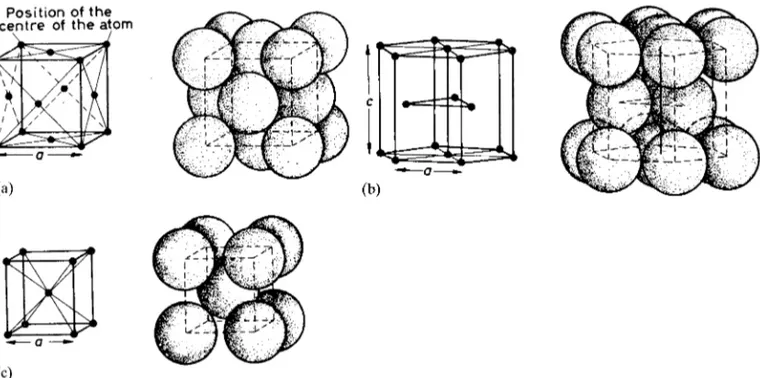
2.5.1 Pure metals 18
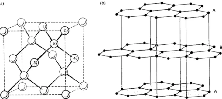
2.5.2 Diamond and graphite 21 2.5.3 Coordination in ionic crystals 22 2.5.4 AB-type compounds 24
2.5.5 Silica 24 2.5.6 Alumina 26 2.5.7 Complex oxides 26 2.5.8 Silicates 27 2.6 Inorganic glasses 30
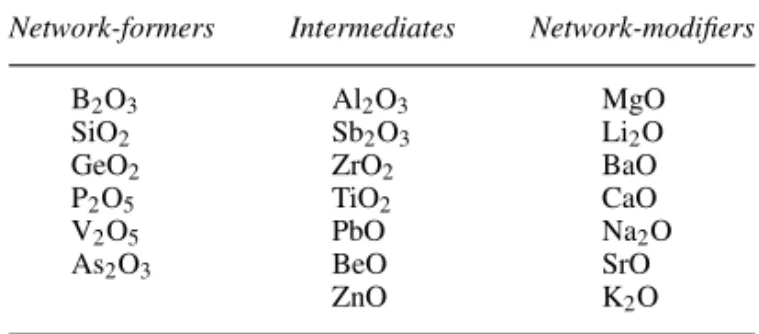
2.6.1 Network structures in glasses 30 2.6.2 Classification of constituent
oxides 31 2.7 Polymeric structures 32
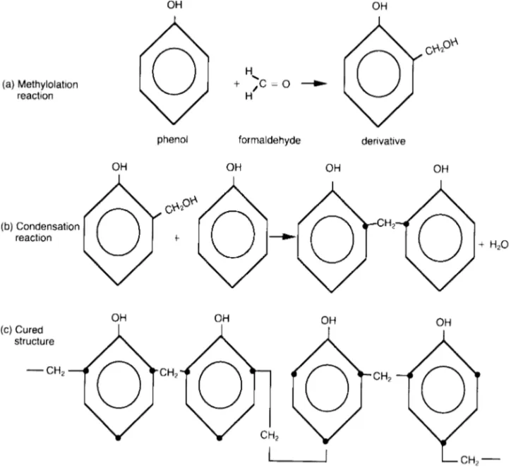
2.7.1 Thermoplastics 32 2.7.2 Elastomers 35 2.7.3 Thermosets 36
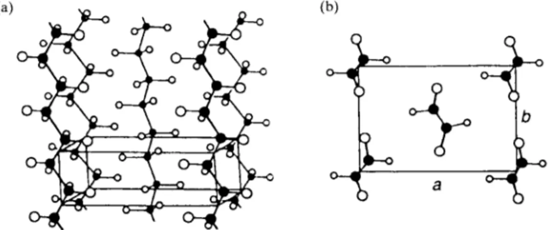
2.7.4 Crystallinity in polymers 38
3 Structural phases; their formation and transitions 42
3.1 Crystallization from the melt 42 3.1.1 Freezing of a pure metal 42 3.1.2 Plane-front and dendritic
solidification at a cooled surface 43
3.1.3 Forms of cast structure 44 3.1.4 Gas porosity and segregation 45 3.1.5 Directional solidification 46 3.1.6 Production of metallic single crystals
for research 47
3.2 Principles and applications of phase diagrams 48
3.2.1 The concept of a phase 48 3.2.2 The Phase Rule 48 3.2.3 Stability of phases 49 3.2.4 Two-phase equilibria 52 3.2.5 Three-phase equilibria and
reactions 56
3.2.6 Intermediate phases 58
3.2.7 Limitations of phase diagrams 59 3.2.8 Some key phase diagrams 60 3.2.9 Ternary phase diagrams 64 3.3 Principles of alloy theory 73
3.3.1 Primary substitutional solid solutions 73
3.3.2 Interstitial solid solutions 76 3.3.3 Types of intermediate phases 76 3.3.4 Order-disorder phenomena 79 3.4 The mechanism of phase changes 80
3.4.1 Kinetic considerations 80 3.4.2 Homogeneous nucleation 81 3.4.3 Heterogeneous nucleation 82 3.4.4 Nucleation in solids 82
4 Defects in solids 84
vi Contents
4.2 Point defects 84
4.2.1 Point defects in metals 84 4.2.2 Point defects in non-metallic
crystals 86
4.2.3 Irradiation of solids 87 4.2.4 Point defect concentration and
annealing 89 4.3 Line defects 90
4.3.1 Concept of a dislocation 90 4.3.2 Edge and screw dislocations 91 4.3.3 The Burgers vector 91
4.3.4 Mechanisms of slip and climb 92 4.3.5 Strain energy associated with
dislocations 95
4.3.6 Dislocations in ionic structures 97 4.4 Planar defects 97
4.4.1 Grain boundaries 97 4.4.2 Twin boundaries 98
4.4.3 Extended dislocations and stacking faults in close-packed crystals 99 4.5 Volume defects 104
4.5.1 Void formation and annealing 104 4.5.2 Irradiation and voiding 104 4.5.3 Voiding and fracture 104 4.6 Defect behaviour in some real
materials 105
4.6.1 Dislocation vector diagrams and the Thompson tetrahedron 105 4.6.2 Dislocations and stacking faults in
fcc structures 106
4.6.3 Dislocations and stacking faults in cph structures 108
4.6.4 Dislocations and stacking faults in bcc structures 112
4.6.5 Dislocations and stacking faults in ordered structures 113
4.6.6 Dislocations and stacking faults in ceramics 115
4.6.7 Defects in crystalline polymers 116 4.6.8 Defects in glasses 117 4.7 Stability of defects 117
4.7.1 Dislocation loops 117 4.7.2 Voids 119
4.7.3 Nuclear irradiation effects 119
5 The characterization of materials 125 5.1 Tools of characterization 125 5.2 Light microscopy 126
5.2.1 Basic principles 126 5.2.2 Selected microscopical
techniques 127 5.3 X-ray diffraction analysis 133
5.3.1 Production and absorption of X-rays 133
5.3.2 Diffraction of X-rays by crystals 134
5.3.3 X-ray diffraction methods 135 5.3.4 Typical interpretative procedures for
diffraction patterns 138 5.4 Analytical electron microscopy 142
5.4.1 Interaction of an electron beam with a solid 142
5.4.2 The transmission electron microscope (TEM) 143 5.4.3 The scanning electron
microscope 144
5.4.4 Theoretical aspects of TEM 146 5.4.5 Chemical microanalysis 150 5.4.6 Electron energy loss spectroscopy
(EELS) 152
5.4.7 Auger electron spectroscopy (AES) 154
5.5 Observation of defects 154 5.5.1 Etch pitting 154
5.5.2 Dislocation decoration 155 5.5.3 Dislocation strain contrast in
TEM 155
5.5.4 Contrast from crystals 157 5.5.5 Imaging of dislocations 157 5.5.6 Imaging of stacking faults 158 5.5.7 Application of dynamical
theory 158
5.5.8 Weak-beam microscopy 160 5.6 Specialized bombardment techniques 161
5.6.1 Neutron diffraction 161
5.6.2 Synchrotron radiation studies 162 5.6.3 Secondary ion mass spectrometry
(SIMS) 163 5.7 Thermal analysis 164
5.7.1 General capabilities of thermal analysis 164
5.7.2 Thermogravimetric analysis 164 5.7.3 Differential thermal analysis 165 5.7.4 Differential scanning
calorimetry 165
6 The physical properties of materials 168 6.1 Introduction 168
6.2 Density 168
6.3 Thermal properties 168 6.3.1 Thermal expansion 168 6.3.2 Specific heat capacity 170 6.3.3 The specific heat curve and
transformations 171
6.3.4 Free energy of transformation 171 6.4 Diffusion 172
6.4.1 Diffusion laws 172
6.4.2 Mechanisms of diffusion 174 6.4.3 Factors affecting diffusion 175 6.5 Anelasticity and internal friction 176 6.6 Ordering in alloys 177
Contents vii
6.6.2 Detection of ordering 178 6.6.3 Influence of ordering upon
properties 179 6.7 Electrical properties 181
6.7.1 Electrical conductivity 181 6.7.2 Semiconductors 183 6.7.3 Superconductivity 185 6.7.4 Oxide superconductors 187 6.8 Magnetic properties 188
6.8.1 Magnetic susceptibility 188 6.8.2 Diamagnetism and
paramagnetism 189 6.8.3 Ferromagnetism 189 6.8.4 Magnetic alloys 191 6.8.5 Anti-ferromagnetism and
ferrimagnetism 192 6.9 Dielectric materials 193
6.9.1 Polarization 193
6.9.2 Capacitors and insulators 193 6.9.3 Piezoelectric materials 194 6.9.4 Pyroelectric and ferroelectric
materials 194 6.10 Optical properties 195
6.10.1 Reflection, absorption and transmission effects 195 6.10.2 Optical fibres 195 6.10.3 Lasers 195
6.10.4 Ceramic ‘windows’ 196 6.10.5 Electro-optic ceramics 196
7 Mechanical behaviour of materials 197 7.1 Mechanical testing procedures 197
7.1.1 Introduction 197 7.1.2 The tensile test 197
7.1.3 Indentation hardness testing 199 7.1.4 Impact testing 199
7.1.5 Creep testing 199 7.1.6 Fatigue testing 200 7.1.7 Testing of ceramics 200 7.2 Elastic deformation 201
7.2.1 Elastic deformation of metals 201 7.2.2 Elastic deformation of
ceramics 203 7.3 Plastic deformation 203
7.3.1 Slip and twinning 203 7.3.2 Resolved shear stress 203 7.3.3 Relation of slip to crystal
structure 204
7.3.4 Law of critical resolved shear stress 205
7.3.5 Multiple slip 205
7.3.6 Relation between work-hardening and slip 206
7.4 Dislocation behaviour during plastic deformation 207
7.4.1 Dislocation mobility 207
7.4.2 Variation of yield stress with temperature and strain rate 208 7.4.3 Dislocation source operation 209 7.4.4 Discontinuous yielding 211 7.4.5 Yield points and crystal
structure 212
7.4.6 Discontinuous yielding in ordered alloys 214
7.4.7 Solute–dislocation interaction 214 7.4.8 Dislocation locking and
temperature 216
7.4.9 Inhomogeneity interaction 217 7.4.10 Kinetics of strain-ageing 217 7.4.11 Influence of grain boundaries on
plasticity 218 7.4.12 Superplasticity 220 7.5 Mechanical twinning 221
7.5.1 Crystallography of twinning 221 7.5.2 Nucleation and growth of
twins 222
7.5.3 Effect of impurities on twinning 223
7.5.4 Effect of prestrain on twinning 223 7.5.5 Dislocation mechanism of
twinning 223
7.5.6 Twinning and fracture 224 7.6 Strengthening and hardening
mechanisms 224
7.6.1 Point defect hardening 224 7.6.2 Work-hardening 226 7.6.3 Development of preferred
orientation 232 7.7 Macroscopic plasticity 235
7.7.1 Tresca and von Mises criteria 235 7.7.2 Effective stress and strain 236 7.8 Annealing 237
7.8.1 General effects of annealing 237 7.8.2 Recovery 237
7.8.3 Recrystallization 239 7.8.4 Grain growth 242 7.8.5 Annealing twins 243 7.8.6 Recrystallization textures 245 7.9 Metallic creep 245
7.9.1 Transient and steady-state creep 245
7.9.2 Grain boundary contribution to creep 247
7.9.3 Tertiary creep and fracture 249 7.9.4 Creep-resistant alloy design 249 7.10 Deformation mechanism maps 251 7.11 Metallic fatigue 252
7.11.1 Nature of fatigue failure 252 7.11.2 Engineering aspects of fatigue 252 7.11.3 Structural changes accompanying
fatigue 254
viii Contents
7.11.5 Fatigue at elevated temperatures 258
8 Strengthening and toughening 259 8.1 Introduction 259
8.2 Strengthening of non-ferrous alloys by heat-treatment 259
8.2.1 Precipitation-hardening of Al –Cu alloys 259
8.2.2 Precipitation-hardening of Al –Ag alloys 263
8.2.3 Mechanisms of
precipitation-hardening 265 8.2.4 Vacancies and precipitation 268 8.2.5 Duplex ageing 271
8.2.6 Particle-coarsening 272 8.2.7 Spinodal decomposition 273 8.3 Strengthening of steels by
heat-treatment 274
8.3.1 Time–temperature–transformation diagrams 274
8.3.2 Austenite–pearlite transformation 276 8.3.3 Austenite–martensite transformation 278 8.3.4 Austenite–bainite
transformation 282
8.3.5 Tempering of martensite 282 8.3.6 Thermo-mechanical
treatments 283 8.4 Fracture and toughness 284
8.4.1 Griffith micro-crack criterion 284 8.4.2 Fracture toughness 285
8.4.3 Cleavage and the ductile–brittle transition 288
8.4.4 Factors affecting brittleness of steels 289
8.4.5 Hydrogen embrittlement of steels 291
8.4.6 Intergranular fracture 291 8.4.7 Ductile failure 292 8.4.8 Rupture 293
8.4.9 Voiding and fracture at elevated temperatures 293
8.4.10 Fracture mechanism maps 294 8.4.11 Crack growth under fatigue
conditions 295
9 Modern alloy developments 297 9.1 Introduction 297
9.2 Commercial steels 297 9.2.1 Plain carbon steels 297 9.2.2 Alloy steels 298 9.2.3 Maraging steels 299
9.2.4 High-strength low-alloy (HSLA) steels 299
9.2.5 Dual-phase (DP) steels 300
9.2.6 Mechanically alloyed (MA) steels 301
9.2.7 Designation of steels 302 9.3 Cast irons 303
9.4 Superalloys 305
9.4.1 Basic alloying features 305 9.4.2 Nickel-based superalloy
development 306 9.4.3 Dispersion-hardened
superalloys 307 9.5 Titanium alloys 308
9.5.1 Basic alloying and heat-treatment features 308
9.5.2 Commercial titanium alloys 310 9.5.3 Processing of titanium alloys 312 9.6 Structural intermetallic compounds 312
9.6.1 General properties of intermetallic compounds 312
9.6.2 Nickel aluminides 312 9.6.3 Titanium aluminides 314
9.6.4 Other intermetallic compounds 315 9.7 Aluminium alloys 316
9.7.1 Designation of aluminium alloys 316
9.7.2 Applications of aluminium alloys 316
9.7.3 Aluminium-lithium alloys 317 9.7.4 Processing developments 317
10 Ceramics and glasses 320
10.1 Classification of ceramics 320 10.2 General properties of ceramics 321 10.3 Production of ceramic powders 322 10.4 Selected engineering ceramics 323
10.4.1 Alumina 323
10.4.2 From silicon nitride to sialons 325 10.4.3 Zirconia 330
10.4.4 Glass-ceramics 331 10.4.5 Silicon carbide 334 10.4.6 Carbon 337
10.5 Aspects of glass technology 345 10.5.1 Viscous deformation of glass 345 10.5.2 Some special glasses 346 10.5.3 Toughened and laminated
glasses 346
10.6 The time-dependency of strength in ceramics and glasses 348
11 Plastics and composites 351
11.1 Utilization of polymeric materials 351 11.1.1 Introduction 351
11.1.2 Mechanical aspects ofTg 351 11.1.3 The role of additives 352 11.1.4 Some applications of important
plastics 353
Contents ix
11.2 Behaviour of plastics during processing 355
11.2.1 Cold-drawing and crazing 355 11.2.2 Processing methods for
thermoplastics 356
11.2.3 Production of thermosets 357 11.2.4 Viscous aspects of melt
behaviour 358 11.2.5 Elastic aspects of melt
behaviour 359 11.2.6 Flow defects 360
11.3 Fibre-reinforced composite materials 361 11.3.1 Introduction to basic structural
principles 361
11.3.2 Types of fibre-reinforced composite 366
12 Corrosion and surface engineering 376
12.1 The engineering importance of surfaces 376
12.2 Metallic corrosion 376
12.2.1 Oxidation at high temperatures 376 12.2.2 Aqueous corrosion 382
12.3 Surface engineering 387
12.3.1 The coating and modification of surfaces 387
12.3.2 Surface coating by vapour deposition 388
12.3.3 Surface coating by particle bombardment 391 12.3.4 Surface modification with
high-energy beams 391
13 Biomaterials 394 13.1 Introduction 394
13.2 Requirements for biomaterials 394 13.3 Dental materials 395
13.3.1 Cavity fillers 395
13.3.2 Bridges, crowns and dentures 396 13.3.3 Dental implants 397
13.4 The structure of bone and bone fractures 397
13.5 Replacement joints 398 13.5.1 Hip joints 398 13.5.2 Shoulder joints 399 13.5.3 Knee joints 399
13.5.4 Finger joints and hand surgery 399 13.6 Reconstructive surgery 400
13.6.1 Plastic surgery 400 13.6.2 Maxillofacial surgery 401 13.6.3 Ear implants 402 13.7 Biomaterials for heart repair 402
13.7.1 Heart valves 402
13.7.2 Pacemakers 403 13.7.3 Artificial arteries 403 13.8 Tissue repair and growth 403 13.9 Other surgical applications 404 13.10 Ophthalmics 404
13.11 Drug delivery systems 405
14 Materials for sports 406
14.1 The revolution in sports products 406 14.2 The tradition of using wood 406 14.3 Tennis rackets 407
14.3.1 Frames for tennis rackets 407 14.3.2 Strings for tennis rackets 408 14.4 Golf clubs 409
14.4.1 Kinetic aspects of a golf stroke 409
14.4.2 Golf club shafts 410 14.4.3 Wood-type club heads 410 14.4.4 Iron-type club heads 411 14.4.5 Putting heads 411 14.5 Archery bows and arrows 411
14.5.1 The longbow 411 14.5.2 Bow design 411 14.5.3 Arrow design 412 14.6 Bicycles for sport 413
14.6.1 Frame design 413
14.6.2 Joining techniques for metallic frames 414
14.6.3 Frame assembly using epoxy adhesives 414
14.6.4 Composite frames 415 14.6.5 Bicycle wheels 415 14.7 Fencing foils 415
14.8 Materials for snow sports 416 14.8.1 General requirements 416 14.8.2 Snowboarding equipment 416 14.8.3 Skiing equipment 417 14.9 Safety helmets 417
14.9.1 Function and form of safety helmets 417
14.9.2 Mechanical behaviour of foams 418
14.9.3 Mechanical testing of safety helmets 418
Appendices 420 1 SI units 420
2 Conversion factors, constants and physical data 422
Figure references 424
Preface
It is less than five years since the last edition of Modern Physical Metallurgy was enlarged to include the related subject of Materials Science and Engi-neering, appearing under the title Metals and Mate-rials: Science, Processes, Applications. In its revised approach, it covered a wider range of metals and alloys and included ceramics and glasses, polymers and composites, modern alloys and surface engineer-ing. Each of these additional subject areas was treated on an individual basis as well as against unifying background theories of structure, kinetics and phase transformations, defects and materials characteriza-tion.
In the relatively short period of time since that previous edition, there have been notable advances in the materials science and engineering of biomat-erials and sports equipment. Two new chapters have now been devoted to these topics. The subject of biomaterials concerns the science and application of materials that must function effectively and reliably whilst in contact with living tissue; these vital mat-erials feature increasingly in modern surgery, medicine and dentistry. Materials developed for sports equip-ment must take into account the demands peculiar to each sport. In the process of writing these addi-tional chapters, we became increasingly conscious that engineering aspects of the book were coming more and more into prominence. A new form of title was deemed appropriate. Finally, we decided to combine the phrase ‘physical metallurgy’, which expresses a sense of continuity with earlier edi-tions, directly with ‘materials engineering’ in the book’s title.
Overall, as in the previous edition, the book aims to present the science of materials in a relatively concise form and to lead naturally into an explanation of the ways in which various important materials are pro-cessed and applied. We have sought to provide a useful survey of key materials and their interrelations, empha-sizing, wherever possible, the underlying scientific and engineering principles. Throughout we have indicated the manner in which powerful tools of characteriza-tion, such as optical and electron microscopy, X-ray diffraction, etc. are used to elucidate the vital relations between the structure of a material and its mechani-cal, physical and/or chemical properties. Control of the microstructure/property relation recurs as a vital theme during the actual processing of metals, ceramics and polymers; production procedures for ostensibly dissim-ilar materials frequently share common principles.
We have continued to try and make the subject area accessible to a wide range of readers. Sufficient background and theory is provided to assist students in answering questions over a large part of a typical Degree course in materials science and engineering. Some sections provide a background or point of entry for research studies at postgraduate level. For the more general reader, the book should serve as a useful introduction or occasional reference on the myriad ways in which materials are utilized. We hope that we have succeeded in conveying the excitement of the atmosphere in which a life-altering range of new materials is being conceived and developed.
Chapter 1
The structure and bonding of atoms
1.1 The realm of materials science
In everyday life we encounter a remarkable range of engineering materials: metals, plastics and ceramics are some of the generic terms that we use to describe them. The size of the artefact may be extremely small, as in the silicon microchip, or large, as in the welded steel plate construction of a suspension bridge. We acknowledge that these diverse materials are quite lit-erally the stuff of our civilization and have a deter-mining effect upon its character, just as cast iron did during the Industrial Revolution. The ways in which we use, or misuse, materials will obviously also influ-ence its future. We should recognize that the pressing and interrelated global problems of energy utilization and environmental control each has a substantial and inescapable ‘materials dimension’.The engineer is primarily concerned with the func-tion of the component or structure, frequently with its capacity to transmit working stresses without risk of failure. The secondary task, the actual choice of a suitable material, requires that the materials scientist should provide the necessary design data, synthesize and develop new materials, analyse fail-ures and ultimately produce material with the desired shape, form and properties at acceptable cost. This essential collaboration between practitioners of the two disciplines is sometimes expressed in the phrase ‘Materials Science and Engineering (MSE)’. So far as the main classes of available materials are con-cerned, it is initially useful to refer to the type of diagram shown in Figure 1.1. The principal sectors represent metals, ceramics and polymers. All these materials can now be produced in non-crystalline forms, hence a glassy ‘core’ is shown in the diagram. Combining two or more materials of very different properties, a centuries-old device, produces important composite materials: carbon-fibre-reinforced polymers (CFRP) and metal-matrix composites (MMC) are mod-ern examples.
Figure 1.1 The principal classes of materials (after Rice, 1983).
2 Modern Physical Metallurgy and Materials Engineering
Having outlined the place of materials science in our highly material-dependent civilization, it is now appropriate to consider the smallest structural entity in materials and its associated electronic states.
1.2 The free atom
1.2.1 The four electron quantum numbers
Rutherford conceived the atom to be a positively-charged nucleus, which carried the greater part of the mass of the atom, with electrons clustering around it. He suggested that the electrons were revolving round the nucleus in circular orbits so that the centrifugal force of the revolving electrons was just equal to the electrostatic attraction between the positively-charged nucleus and the negatively-charged electrons. In order to avoid the difficulty that revolving electrons should, according to the classical laws of electrodynamics, emit energy continuously in the form of electromag-netic radiation, Bohr, in 1913, was forced to conclude that, of all the possible orbits, only certain orbits were in fact permissible. These discrete orbits were assumed to have the remarkable property that when an elec-tron was in one of these orbits, no radiation could take place. The set of stable orbits was characterized by the criterion that the angular momenta of the electrons in the orbits were given by the expressionnh/2, where his Planck’s constant andncould only have integral values (nD1,2,3, etc.). In this way, Bohr was able to give a satisfactory explanation of the line spectrum of the hydrogen atom and to lay the foundation of modern atomic theory.In later developments of the atomic theory, by de Broglie, Schr¨odinger and Heisenberg, it was realized that the classical laws of particle dynamics could not be applied to fundamental particles. In classical dynamics it is a prerequisite that the position and momentum of a particle are known exactly: in atomic dynamics, if either the position or the momentum of a fundamental particle is known exactly, then the other quantity cannot be determined. In fact, an uncertainty must exist in our knowledge of the position and momentum of a small particle, and the product of the degree of uncertainty for each quantity is related to the value of Planck’s constant⊲hD6.6256ð1034 J s⊳. In the macroscopic world, this fundamental uncertainty is too small to be measurable, but when treating the motion of electrons revolving round an atomic nucleus, application of Heisenberg’s Uncertainty Principle is essential.
The consequence of the Uncertainty Principle is that we can no longer think of an electron as moving in a fixed orbit around the nucleus but must consider the motion of the electron in terms of a wave func-tion. This function specifies only the probability of finding one electron having a particular energy in the space surrounding the nucleus. The situation is fur-ther complicated by the fact that the electron behaves not only as if it were revolving round the nucleus
but also as if it were spinning about its own axis. Consequently, instead of specifying the motion of an electron in an atom by a single integern, as required by the Bohr theory, it is now necessary to specify the electron state using four numbers. These numbers, known as electron quantum numbers, aren,l,mand
s, wheren is the principal quantum number,l is the orbital (azimuthal) quantum number,mis the magnetic quantum number and s is the spin quantum number. Another basic premise of the modern quantum theory of the atom is the Pauli Exclusion Principle. This states that no two electrons in the same atom can have the same numerical values for their set of four quantum numbers.
If we are to understand the way in which the Periodic Table of the chemical elements is built up in terms of the electronic structure of the atoms, we must now consider the significance of the four quantum numbers and the limitations placed upon the numerical values that they can assume. The most important quantum number is the principal quantum number since it is mainly responsible for determining the energy of the electron. The principal quantum number can have integral values beginning withnD1, which is the state of lowest energy, and electrons having this value are the most stable, the stability decreasing asnincreases. Electrons having a principal quantum number n can take up integral values of the orbital quantum numberlbetween 0 and⊲n1⊳. Thus ifnD1, lcan only have the value 0, while for
nD2,lD0 or 1, and fornD3, lD0, 1 or 2. The orbital quantum number is associated with the angular momentum of the revolving electron, and determines what would be regarded in non-quantum mechanical terms as the shape of the orbit. For a given value of
n, the electron having the lowest value oflwill have the lowest energy, and the higher the value of l, the greater will be the energy.
The remaining two quantum numbers m ands are concerned, respectively, with the orientation of the electron’s orbit round the nucleus, and with the ori-entation of the direction of spin of the electron. For a given value ofl, an electron may have integral values of the inner quantum number m from Cl through 0 tol. Thus forlD2, mcan take on the values C2, C1, 0,1 and 2. The energies of electrons having the same values of n and l but different values of
m are the same, provided there is no magnetic field present. When a magnetic field is applied, the energies of electrons having differentmvalues will be altered slightly, as is shown by the splitting of spectral lines in the Zeeman effect. The spin quantum numbers may, for an electron having the same values ofn,landm, take one of two values, that is, C1
2 or 1
The structure and bonding of atoms 3
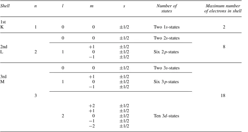
Table 1.1 Allocation of states in the first three quantum shells
Shell n l m s Number of Maximum number
states of electrons in shell
1st
K 1 0 0 š1/2 Two 1s-states 2
0 0 š1/2 Two 2s-states
2nd C1 š1/2 8
L 2 1 0 š1/2 Six 2p-states
1 š1/2
0 0 š1/2 Two 3s-states
3rd C1 š1/2
M 1 0 š1/2 Six 3p-states
1 š1/2
3 18
C2 š1/2
C1 š1/2
2 0 š1/2 Ten 3d-states
1 š1/2
2 š1/2
energies of the two electrons of opposite spin be dif-ferent.
1.2.2 Nomenclature for the electronic states
Before discussing the way in which the periodic clas-sification of the elements can be built up in terms of the electronic structure of the atoms, it is necessary to outline the system of nomenclature which enables us to describe the states of the electrons in an atom. Since the energy of an electron is mainly determined by the values of the principal and orbital quantum numbers, it is only necessary to consider these in our nomenclature. The principal quantum number is sim-ply expressed by giving that number, but the orbital quantum number is denoted by a letter. These letters, which derive from the early days of spectroscopy, ares,p,dandf, which signify that the orbital quantum numberslare 0, 1, 2 and 3, respectively.1
When the principal quantum numbernD1,lmust be equal to zero, and an electron in this state would be designated by the symbol 1s. Such a state can only have a single value of the inner quantum number
mD0, but can have values ofC1 2 or
1
2 for the spin quantum number s. It follows, therefore, that there are only two electrons in any one atom which can be in a 1s-state, and that these electrons will spin in opposite directions. Thus when nD1, only s-states 1The letters,s,p,dandfarose from a classification of
spectral lines into four groups, termed sharp, principal, diffuse and fundamental in the days before the present quantum theory was developed.
can exist and these can be occupied by only two electrons. Once the two 1s-states have been filled, the next lowest energy state must have nD2. Here
l may take the value 0 or 1, and therefore electrons can be in either a 2s-or a 2p-state. The energy of an electron in the 2s-state is lower than in a 2p -state, and hence the 2s-states will be filled first. Once more there are only two electrons in the 2s-state, and indeed this is always true ofs-states, irrespective of the value of the principal quantum number. The electrons in the p-state can have values of mD C1, 0, 1, and electrons having each of these values for m can have two values of the spin quantum number, leading therefore to the possibility of six electrons being in any one p-state. These relationships are shown more clearly in Table 1.1.
No further electrons can be added to the state for
nD2 after two 2s- and six 2p-state are filled, and the next electron must go into the state for which
nD3, which is at a higher energy. Here the possibility arises forl to have the values 0, 1 and 2 and hence, besidess- andp-states,d-states for which lD2 can now occur. When lD2, m may have the values C2,C1,0,1,2 and each may be occupied by two electrons of opposite spin, leading to a total of tend -states. Finally, when nD4, l will have the possible values from 0 to 4, and when lD4 the reader may verify that there are fourteen 4f-states.
4 Modern Physical Metallurgy and Materials Engineering
1.3 The Periodic Table
The Periodic Table provides an invaluable classifi-cation of all chemical elements, an element being a collection of atoms of one type. A typical version is shown in Table 1.2. Of the 107 elements which appear, about 90 occur in nature; the remainder are produced in nuclear reactors or particle accelerators. The atomic number (Z) of each element is stated, together with its chemical symbol, and can be regarded as either the number of protons in the nucleus or the num-ber of orbiting electrons in the atom. The elements are naturally classified into periods (horizontal rows), depending upon which electron shell is being filled, and groups (vertical columns). Elements in any one group have the electrons in their outermost shell in the same configuration, and, as a direct result, have similar chemical properties.
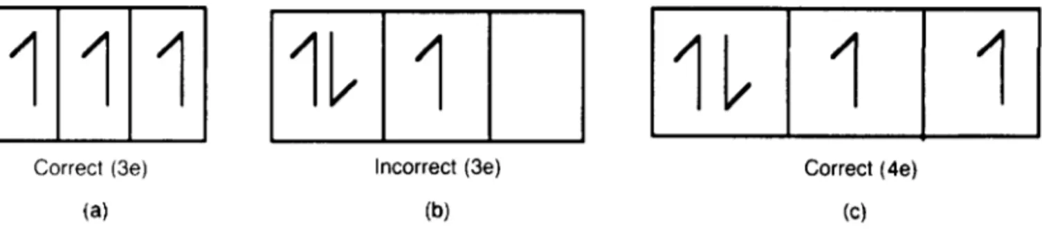
The building principle (Aufbauprinzip) for the Table is based essentially upon two rules. First, the Pauli Exclusion Principle (Section 1.2.1) must be obeyed. Second, in compliance with Hund’s rule of max-imum multiplicity, the ground state should always develop maximum spin. This effect is demonstrated diagrammatically in Figure 1.2. Suppose that we sup-ply three electrons to the three ‘empty’ 2p-orbitals. They will build up a pattern of parallel spins (a) rather than paired spins (b). A fourth electron will cause pairing (c). Occasionally, irregularities occur in the ‘filling’ sequence for energy states because electrons always enter the lowest available energy state. Thus, 4s-states, being at a lower energy level, fill before the 3d-states.
We will now examine the general process by which the Periodic Table is built up, electron by electron, in closer detail. The progressive filling of energy states can be followed in Table 1.3. The first period com-mences with the simple hydrogen atom which has a single proton in the nucleus and a single orbiting elec-tron ⊲ZD1⊳. The atom is therefore electrically neu-tral and for the lowest energy condition, the electron will be in the 1s-state. In helium, the next element, the nucleus charge is increased by one proton and an additional electron maintains neutrality ⊲ZD2⊳. These two electrons fill the 1s-state and will nec-essarily have opposite spins. The nucleus of helium contains two neutrons as well as two protons, hence
its mass is four times greater than that of hydrogen. The next atom, lithium, has a nuclear charge of three
⊲ZD3⊳and, because the first shell is full, an electron must enter the 2s-state which has a somewhat higher energy. The electron in the 2s-state, usually referred to as the valency electron, is ‘shielded’ by the inner electrons from the attracting nucleus and is therefore less strongly bonded. As a result, it is relatively easy to separate this valency electron. The ‘electron core’ which remains contains two tightly-bound electrons and, because it carries a single net positive charge, is referred to as a monovalent cation. The overall pro-cess by which electron(s) are lost or gained is known as ionization.
The development of the first short period from lithium (ZD3) to neon (ZD10) can be conveniently followed by referring to Table 1.3. So far, the sets of states corresponding to two principal quantum num-bers (nD1,nD2) have been filled and the electrons in these states are said to have formed closed shells. It is a consequence of quantum mechanics that, once a shell is filled, the energy of that shell falls to a very low value and the resulting electronic configuration is very stable. Thus, helium, neon, argon and krypton are asso-ciated with closed shells and, being inherently stable and chemically unreactive, are known collectively as the inert gases.
The second short period, from sodium⊲ZD11⊳to argon ⊲ZD18⊳, commences with the occupation of the 3s-orbital and ends when the 3p-orbitals are full (Table 1.3). The long period which follows extends from potassium⊲ZD19⊳to krypton⊲ZD36⊳, and, as mentioned previously, has the unusual feature of the 4s-state filling before the 3d-state. Thus, potassium has a similarity to sodium and lithium in that the electron of highest energy is in an s-state; as a consequence, they have very similar chemical reactivities, forming the group known as the alkali-metal elements. After calcium⊲ZD20⊳, filling of the 3d-state begins.
The 4s-state is filled in calcium ⊲ZD20⊳ and the filling of the 3d-state becomes energetically favourable to give scandium ⊲ZD21⊳. This belated filling of the five 3d-orbitals from scandium to its completion in copper ⊲ZD29⊳ embraces the first series of transition elements. One member of this series, chromium ⊲ZD24⊳, obviously behaves in an unusual manner. Applying Hund’s rule, we can reason
Table 1.2 The Periodic Table of the elements (from Puddephatt and Monaghan, 1986; by permission of Oxford University Press)
1 2 3 4 5 6 7 8 9 10 11 12 13 14 15 16 17 18 New IUPAC notation
IA IIA IIIA IVA VA VIA VIIA VIII IB IIB IIIB IVB VB VIB VIIB O Previous IUPAC form
1H 1.008 2He 4.003 3Li 6.941 4Be 9.012 5B 10.81 6C 12.01 7N 14.01 8O 16.00 9F 19.00 10Ne 20.18 11Na 22.99 12Mg 24.31 13Al 26.98 14Si 28.09 15P 30.97 16S 32.45 17Cl 35.45 18A 39.95 19K 39.10 20Ca 40.08 21Sc 44.96 22Ti 47.90 23V 50.94 24Cr 52.00 25Mn 54.94 26Fe 55.85 27Co 58.93 28Ni 58.71 29Cu 63.55 30Zn 65.37 31Ga 69.72 32Ge 72.92 33Ge 74.92 34Se 78.96 35Br 79.90 36Kr 83.80 37Rb 85.47 38Sr 87.62 39Y 88.91 40Zr 91.22 41Nb 92.91 42Mo 95.94 43Tc 98.91 44Ru 101.1 45Rh 102.9 46Pd 106.4 47Ag 107.9 48Cd 112.4 49In 114.8 50Sn 118.7 51Sb 121.8 52Te 127.6 53I 126.9 54Xe 131.3 55Cs 132.9 56Ba 137.3 57La 138.9 72Hf 178.5 73Ta 180.9 74W 183.9 75Re 186.2 76Os 190.2 77Ir 192.2 78Pt 195.1 79Au 197.0 80Hg 200.6 81Tl 204.4 82Pb 207.2 83Bi 209.0 84Po ⊲210⊳ 85At ⊲210⊳ 86Rn ⊲222⊳ 87Fr ⊲223⊳ 88Ra ⊲226.0⊳ 89Ac ⊲227⊳
104Unq 105Unp 106Unh 107Uns
s-block! d-block! p-block!
Lanthanides 57La 138.9 58Ce 140.1 59Pr 140.9 60Nd 144.2 61Pm ⊲147⊳ 62Sm 150.4 63Eu 152.0 64Gd 157.3 65Tb 158.9 66Dy 162.5 67Ho 164.9 68Er 167.3 69Tm 168.9 70Yb 173.0 71Lu 175.0
6 Modern Physical Metallurgy and Materials Engineering
Table 1.3 Electron quantum numbers (Hume-Rothery, Smallman and Haworth, 1988)
Element and atomic
number Principal and secondary quantum numbers
nD1 2 3 4
lD0 0 1 0 1 2 0 1 2 3
1 H 1 2 He 2 3 Li 2 1 4 Be 2 2 5 B 2 2 1 6 C 2 2 2 7 N 2 2 3 8 O 2 2 4 9 F 2 2 5 10 Ne 2 2 6 11 Na 2 2 6 1 12 Mg 2 2 6 2 13 Al 2 2 6 2 1 14 Si 2 2 6 2 2 15 P 2 2 6 2 3 16 S 2 2 6 2 4 17 Cl 2 2 6 2 5 18 A 2 2 6 2 6 19 K 2 2 6 2 6 1 20 Ca 2 2 6 2 6 2 21 Sc 2 2 6 2 6 1 2 22 Ti 2 2 6 2 6 2 2 23 V 2 2 6 2 6 3 2 24 Cr 2 2 6 2 6 5 1 25 Mn 2 2 6 2 6 5 2 26 Fe 2 2 6 2 6 6 2 27 Co 2 2 6 2 6 7 2 28 Ni 2 2 6 2 6 8 2 29 Cu 2 2 6 2 6 10 1 30 Zn 2 2 6 2 6 10 2 31 Ga 2 2 6 2 6 10 2 1 32 Ge 2 2 6 2 6 10 2 2 33 As 2 2 6 2 6 10 2 3 34 Se 2 2 6 2 6 10 2 4 35 Br 2 2 6 2 6 10 2 5 36 Kr 2 2 6 2 6 10 2 6
nD1 2 3 4 5 6
lD— — — 0 1 2 3 0 1 2 0
37 Rb 2 8 18 2 6 1 38 Sr 2 8 18 2 6 2 39 Y 2 8 18 2 6 1 2 40 Zr 2 8 18 2 6 2 2 41 Nb 2 8 18 2 6 4 1 42 Mo 2 8 18 2 6 5 1 43 Tc 2 8 18 2 6 5 2 44 Ru 2 8 18 2 6 7 1 45 Rh 2 8 18 2 6 8 1 46 Pd 2 8 18 2 6 10 — 47 Ag 2 8 18 2 6 10 1 48 Cd 2 8 18 2 6 10 2 49 In 2 8 18 2 6 10 2 1 50 Sn 2 8 18 2 6 10 2 2 51 Sb 2 8 18 2 6 10 2 3
52 Te 2 8 18 2 6 10 2 4 53 I 2 8 18 2 6 10 2 5 54 Xe 2 8 18 2 6 10 2 6 55 Cs 2 8 18 2 6 10 2 6 1 56 Ba 2 8 18 2 6 10 2 6 2 57 La 2 8 18 2 6 10 2 6 1 2 58 Ce 2 8 18 2 6 10 2 2 6 2 59 Pr 2 8 18 2 6 10 3 2 6 2 60 Nd 2 8 18 2 6 10 4 2 6 2 61 Pm 2 8 18 2 6 10 5 2 6 2 62 Sm 2 8 18 2 6 10 6 2 6 2 63 Eu 2 8 18 2 6 10 7 2 6 2 64 Gd 2 8 18 2 6 10 7 2 6 1 2 65 Tb 2 8 18 2 6 10 9 2 6 2 66 Dy 2 8 18 2 6 10 10 2 6 2 67 Ho 2 8 18 2 6 10 11 2 6 2 68 Er 2 8 18 2 6 10 12 2 6 2 69 Tm 2 8 18 2 6 10 13 2 6 2 70 Yb 2 8 18 2 6 10 14 2 6 2 71 Lu 2 8 18 2 6 10 14 2 6 1 2 72 Hf 2 8 18 2 6 10 14 2 6 2 2
nD1 2 3 4 5 6 7
lD— — — — 0 1 2 3 0 1 2 0
73 Ta 2 8 18 32 2 6 3 2 74 W 2 8 18 32 2 6 4 2 75 Re 2 8 18 32 2 6 5 2 76 Os 2 8 18 32 2 6 6 2 77 Ir 2 8 18 32 2 6 7 2 78 Pt 2 8 18 32 2 6 9 1 79 Au 2 8 18 32 2 6 10 1 80 Hg 2 8 18 32 2 6 10 2 81 Tl 2 8 18 32 2 6 10 2 1 82 Pb 2 8 18 32 2 6 10 2 2 83 Bi 2 8 18 32 2 6 10 2 3 84 Po 2 8 18 32 2 6 10 2 4 85 At 2 8 18 32 2 6 10 2 5 86 Rn 2 8 18 32 2 6 10 2 6 87 Fr 2 8 18 32 2 6 10 2 6 1 88 Ra 2 8 18 32 2 6 10 2 6 2 89 Ac 2 8 18 32 2 6 10 2 6 1 2 90 Th 2 18 8 32 2 6 10 2 6 2 2 91 Pa 2 18 8 32 2 6 10 2 2 6 1 2 92 U 2 18 8 32 2 6 10 3 2 6 1 2 93 Np 2 18 8 32 2 6 10 4 2 6 1 2 94 Pu 2 18 8 32 2 6 10 5 2 6 1 2
The exact electronic configurations of the later elements are not always certain but the most probable arrangements of the outer electrons are:
95 Am ⊲5f⊳7⊲7s⊳2
96 Cm ⊲5f⊳7⊲6d⊳1⊲7s⊳2
97 Bk ⊲5f⊳8⊲6d⊳1⊲7s⊳2
98 Cf ⊲5f⊳10⊲7s⊳2
99 Es ⊲5f⊳11⊲7s⊳2
100 Fm ⊲5f⊳12⊲7s⊳2
101 Md ⊲5f⊳13⊲7s⊳2
102 No ⊲5f⊳14⊲7s⊳2
103 Lw ⊲5f⊳14⊲6d⊳1⊲7s⊳2
The structure and bonding of atoms 7
that maximization of parallel spin is achieved by locating six electrons, of like spin, so that five fill the 3d-states and one enters the 4s-state. This mode of fully occupying the 3d-states reduces the energy of the electrons in this shell considerably. Again, in copper ⊲ZD29⊳, the last member of this transition series, complete filling of all 3d-orbitals also produces a significant reduction in energy. It follows from these explanations that the 3d- and 4s-levels of energy are very close together. After copper, the energy states fill in a straightforward manner and the first long period finishes with krypton ⊲ZD36⊳. It will be noted that lanthanides (ZD57 to 71) and actinides (ZD89 to 103), because of their state-filling sequences, have been separated from the main body of Table 1.2. Having demonstrated the manner in which quantum rules are applied to the construction of the Periodic Table for the first 36 elements, we can now examine some general aspects of the classification.
When one considers the small step difference of one electron between adjacent elements in the Periodic Table, it is not really surprising to find that the distinction between metallic and non-metallic elements is imprecise. In fact there is an intermediate range of elements, the metalloids, which share the properties of both metals and non-metals. However, we can regard the elements which can readily lose an electron, by ionization or bond formation, as strongly metallic in character (e.g. alkali metals). Conversely, elements which have a strong tendency to acquire an electron and thereby form a stable configuration of two or eight electrons in the outermost shell are non-metallic (e.g. the halogens fluorine, chlorine, bromine, iodine). Thus electropositive metallic elements and the electronegative non-metallic elements lie on the left- and right-hand sides of the Periodic Table, respectively. As will be seen later, these and other aspects of the behaviour of the outermost (valence) electrons have a profound and determining effect upon bonding and therefore upon electrical, magnetic and optical properties.
Prior to the realization that the frequently observed periodicities of chemical behaviour could be expressed in terms of electronic configurations, emphasis was placed upon ‘atomic weight’. This quantity, which is now referred to as relative atomic mass, increases steadily throughout the Periodic Table as protons and neutrons are added to the nuclei. Atomic mass1 determines physical properties such as density, spe-cific heat capacity and ability to absorb electromag-netic radiation: it is therefore very relevant to engi-neering practice. For instance, many ceramics are based upon the light elements aluminium, silicon and oxygen and consequently have a low density, i.e. <3000 kg m3.
1Atomic mass is now expressed relative to the datum value
for carbon (12.01). Thus, a copper atom has 63.55/12.01 or 5.29 times more mass than a carbon atom.
1.4 Interatomic bonding in materials
Matter can exist in three states and as atoms change directly from either the gaseous state (desublimation) or the liquid state (solidification) to the usually denser solid state, the atoms form aggregates in three-dimensional space. Bonding forces develop as atoms are brought into proximity to each other. Sometimes these forces are spatially-directed. The nature of the bonding forces has a direct effect upon the type of solid structure which develops and therefore upon the physical properties of the material. Melting point provides a useful indication of the amount of thermal energy needed to sever these interatomic (or interionic) bonds. Thus, some solids melt at relatively low temperatures (m.p. of tinD232°C) whereas many ceramics melt at extremely high temperatures (m.p. of alumina exceeds 2000°C). It is immediately apparent that bond strength has far-reaching implications in all fields of engineering.Customarily we identify four principal types of bonding in materials, namely, metallic bonding, ionic bonding, covalent bonding and the comparatively much weaker van der Waals bonding. However, in many solid materials it is possible for bonding to be mixed, or even intermediate, in character. We will first consider the general chemical features of each type of bonding; in Chapter 2 we will examine the resultant disposition of the assembled atoms (ions) in three-dimensional space.
As we have seen, the elements with the most pro-nounced metallic characteristics are grouped on the left-hand side of the Periodic Table (Table 1.2). In general, they have a few valence electrons, outside the outermost closed shell, which are relatively easy to detach. In a metal, each ‘free’ valency electron is shared among all atoms, rather than associated with an individual atom, and forms part of the so-called ‘elec-tron gas’ which circulates at random among the regular array of positively-charged electron cores, or cations (Figure 1.3a). Application of an electric potential gra-dient will cause the ‘gas’ to drift though the structure with little hindrance, thus explaining the outstanding electrical conductivity of the metallic state. The metal-lic bond derives from the attraction between the cations and the free electrons and, as would be expected, repul-sive components of force develop when cations are brought into close proximity. However, the bonding forces in metallic structures are spatially non-directed and we can readily simulate the packing and space-filling characteristics of the atoms with modelling sys-tems based on equal-sized spheres (polystyrene balls, even soap bubbles). Other properties such as ductility, thermal conductivity and the transmittance of electro-magnetic radiation are also directly influenced by the non-directionality and high electron mobility of the metallic bond.
8 Modern Physical Metallurgy and Materials Engineering
Figure 1.3 Schematic representation of (a) metallic bonding, (b) ionic bonding, (c) covalent bonding and (d) van der Waals bonding.
of the resultant ions to attain a stable closed shell. For example, the ionic structure of magnesia (MgO), a ceramic oxide, forms when each magnesium atom ⊲ZD12⊳loses two electrons from its L-shell⊲nD2⊳ and these electrons are acquired by an oxygen atom ⊲ZD8⊳, producing a stable octet configuration in its L-shell (Table 1.3). Overall, the ionic charges balance and the structure is electrically neutral (Figure 1.3b). Anions are usually larger than cations. Ionic bonding is omnidirectional, essentially electrostatic in charac-ter and can be extremely strong; for instance, magnesia is a very useful refractory oxide⊲m.p.D2930°C⊳. At low to moderate temperatures, such structures are elec-trical insulators but, typically, become conductive at high temperatures when thermal agitation of the ions increases their mobility.
Sharing of valence electrons is the key feature of the third type of strong primary bonding. Covalent bonds form when valence electrons of opposite spin from adjacent atoms are able to pair within overlapping spatially-directed orbitals, thereby enabling each atom to attain a stable electronic configuration (Figure 1.3c).
Being oriented in three-dimensional space, these local-ized bonds are unlike metallic and ionic bonds. Fur-thermore, the electrons participating in the bonds are tightly bound so that covalent solids, in general, have low electrical conductivity and act as insulators, some-times as semiconductors (e.g. silicon). Carbon in the form of diamond is an interesting prototype for cova-lent bonding. Its high hardness, low coefficient of ther-mal expansion and very high melting point⊲3300°C⊳ bear witness to the inherent strength of the cova-lent bond. First, using the (8 – N) Rule, in which N is the Group Number1 in the Periodic Table, we deduce that carbon⊲ZD6⊳is tetravalent; that is, four bond-forming electrons are available from the L-shell ⊲nD2⊳. In accordance with Hund’s Rule (Figure 1.2), one of the two electrons in the 2s-state is promoted to a higher 2p-state to give a maximum spin condition, pro-ducing an overall configuration of 1s2 2s1 2p3in the carbon atom. The outermost second shell accordingly
1According to previous IUPAC notation: see top of
The structure and bonding of atoms 9
has four valency electrons of like spin available for pairing. Thus each carbon atom can establish electron-sharing orbitals with four neighbours. For a given atom, these four bonds are of equal strength and are set at equal angles⊲109.5°⊳to each other and therefore exhibit tetrahedral symmetry. (The structural conse-quences of this important feature will be discussed in Chapter 2.)
This process by which s-orbitals and p-orbitals combine to form projecting hybridsp-orbitals is known as hybridization. It is observed in elements other than carbon. For instance, trivalent boron ⊲ZD5⊳ forms three co-planarsp2-orbitals. In general, a large degree of overlap ofsp-orbitals and/or a high electron density within the overlap ‘cloud’ will lead to an increase in the strength of the covalent bond. As indicated earlier, it is possible for a material to possess more than one type of bonding. For example, in calcium silicate ⊲Ca2SiO4⊳, calcium cations Ca2Care ionically bonded to tetrahedral SiO44 clusters in which each silicon atom is covalently-bonded to four oxygen neighbours. The final type of bonding is attributed to the van-der Waals forces which develop when adjacent atoms, or groups of atoms, act as electric dipoles. Suppose that two atoms which differ greatly in size combine to form a molecule as a result of covalent bonding. The resultant electron ‘cloud’ for the whole molecule can be pictured as pear-shaped and will have an asymmet-rical distribution of electron charge. An electric dipole has formed and it follows that weak directed forces of electrostatic attraction can exist in an aggregate of such molecules (Figure 1.3d). There are no ‘free’ electrons hence electrical conduction is not favoured. Although secondary bonding by van der Waals forces is weak in comparison to the three forms of primary bonding, it has practical significance. For instance, in the technologically-important mineral talc, which is hydrated magnesium silicate Mg3Si4O10⊲OH⊳2, the parallel covalently-bonded layers of atoms are attracted to each other by van der Waals forces. These layers can easily be slid past each other, giving the mineral its characteristically slippery feel. In thermoplastic poly-mers, van der Waals forces of attraction exist between the extended covalently-bonded hydrocarbon chains; a combination of heat and applied shear stress will over-come these forces and cause the molecular chains to glide past each other. To quote a more general case, molecules of water vapour in the atmosphere each have an electric dipole and will accordingly tend to be adsorbed if they strike solid surfaces possessing attractive van der Waals forces (e.g. silica gel).
1.5 Bonding and energy levels
If one imagines atoms being brought together uni-formly to form, for example, a metallic structure, then when the distance between neighbouring atoms approaches the interatomic value the outer electrons are no longer localized around individual atoms. Once
the outer electrons can no longer be considered to be attached to individual atoms but have become free to move throughout the metal then, because of the Pauli Exclusion Principle, these electrons cannot retain the same set of quantum numbers that they had when they were part of the atoms. As a consequence, the free electrons can no longer have more than two electrons of opposite spin with a particular energy. The energies of the free electrons are distributed over a range which increases as the atoms are brought together to form the metal. If the atoms when brought together are to form a stable metallic structure, it is necessary that the mean energy of the free electrons shall be lower than the energy of the electron level in the free atom from which they are derived. Figure 1.4 shows the broaden-ing of an atomic electron level as the atoms are brought together, and also the attendant lowering of energy of the electrons. It is the extent of the lowering in mean energy of the outer electrons that governs the stability of a metal. The equilibrium spacing between the atoms in a metal is that for which any further decrease in the atomic spacing would lead to an increase in the repul-sive interaction of the positive ions as they are forced into closer contact with each other, which would be greater than the attendant decrease in mean electron energy.
In a metallic structure, the free electrons must, therefore, be thought of as occupying a series of discrete energy levels at very close intervals. Each atomic level which splits into a band contains the same number of energy levels as the number N of atoms in the piece of metal. As previously stated, only two electrons of opposite spin can occupy any one level, so that a band can contain a maximum of 2N electrons. Clearly, in the lowest energy state of the metal all the lower energy levels are occupied.
The energy gap between successive levels is not constant but decreases as the energy of the levels increases. This is usually expressed in terms of the density of electronic states N(E)as a function of the energy E. The quantityN⊲E⊳dEgives the number of
10 Modern Physical Metallurgy and Materials Engineering
energy levels in a small energy interval dE, and for free electrons is a parabolic function of the energy, as shown in Figure 1.5.
Because only two electrons can occupy each level, the energy of an electron occupying a low-energy level cannot be increased unless it is given sufficient energy to allow it to jump to an empty level at the top of the band. The energy1 width of these bands is commonly about 5 or 6 eV and, therefore, considerable energy would have to be put into the metal to excite a low-lying electron. Such energies do not occur at normal temperatures, and only those electrons with energies close to that of the top of the band (known
Figure 1.5 (a) Density of energy levels plotted against energy; (b) filling of energy levels by electrons at absolute zero. At ordinary temperatures some of the electrons are thermally excited to higher levels than that corresponding to Emaxas shown by the broken curve in (a).
1An electron volt is the kinetic energy an electron acquires
in falling freely through a potential difference of 1 volt (1 eVD1.602ð1019 J; 1 eV per
particleD23 050ð4.186 J per mol of particles).
as the Fermi level and surface) can be excited, and therefore only a small number of the free electrons in a metal can take part in thermal processes. The energy of the Fermi levelEF depends on the number of electrons N per unit volume V, and is given by ⊲h2/8m⊳⊲3N/V⊳2/3.
The electron in a metallic band must be thought of as moving continuously through the structure with an energy depending on which level of the band it occupies. In quantum mechanical terms, this motion of the electron can be considered in terms of a wave with a wavelength which is determined by the energy of the electron according to de Broglie’s relationship Dh/mv, wherehis Planck’s constant andmand v are, respectively, the mass and velocity of the moving electron. The greater the energy of the electron, the higher will be its momentummv, and hence the smaller will be the wavelength of the wave function in terms of which its motion can be described. Because the movement of an electron has this wave-like aspect, moving electrons can give rise, like optical waves, to diffraction effects. This property of electrons is used in electron microscopy (Chapter 5).
Further reading
Cottrell, A. H. (1975). Introduction to Metallurgy. Edward Arnold, London.
Huheey, J. E. (1983).Inorganic Chemistry, 3rd edn. Harper and Row, New York.
Hume-Rothery, W., Smallman, R. E. and Haworth, C. W. (1975).The Structure of Metals and Alloys, 5th edn (1988 reprint). Institute of Materials, London.
Puddephatt, R. J. and Monaghan, P. K. (1986).The Periodic Table of the Elements.Clarendon Press, Oxford.
Chapter 2
Atomic arrangements in materials
2.1 The concept of ordering
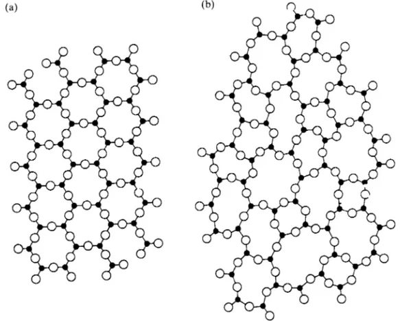
When attempting to classify a material it is useful to decide whether it is crystalline (conventional metals and alloys), non-crystalline (glasses) or a mixture of these two types of structure. The critical distinction between the crystalline and non-crystalline states of matter can be made by applying the concept of ordering. Figure 2.1a shows a symmetrical two-dimensional arrangement of two different types of
atom. A basic feature of this aggregate is the nesting of a small atom within the triangular group of three much larger atoms. This geometrical condition is called short-range ordering. Furthermore, these triangular groups are regularly arranged relative to each other so that if the aggregate were to be extended, we could confidently predict the locations of any added atoms. In effect, we are taking advantage of the long-range ordering characteristic of this array. The array of Figure 2.1a exhibits both short- and long-range
12 Modern Physical Metallurgy and Materials Engineering
ordering and is typical of a single crystal. In the other array of Figure 2.1b, short-range order is discernible but long-range order is clearly absent. This second type of atomic arrangement is typical of the glassy state.1
It is possible for certain substances to exist in either crystalline or glassy forms (e.g. silica). From Figure 2.1 we can deduce that, for such a substance, the glassy state will have the lower bulk density. Furthermore, in comparing the two degrees of ordering of Figures 2.1a and 2.1b, one can appreciate why the structures of comparatively highly-ordered crystalline substances, such as chemical compounds, minerals and metals, have tended to be more amenable to scientific investigation than glasses.
2.2 Crystal lattices and structures
We can rationalize the geometry of the simple repre-sentation of a crystal structure shown in Figure 2.1a by adding a two-dimensional frame of reference, or space lattice, with line intersections at atom centres. Extending this process to three dimensions, we can construct a similar imaginary space lattice in which triple intersections of three families of parallel equidis-tant lines mark the positions of atoms (Figure 2.2a). In this simple case, three reference axes (x, y, z) are oriented at 90° to each other and atoms are ‘shrunk’, for convenience. The orthogonal lattice of Figure 2.2a defines eight unit cells, each having a shared atom at every corner. It follows from our recognition of the inherent order of the lattice that we can express the1The terms glassy, non-crystalline, vitreous and amorphous
are synonymous.
geometrical characteristics of the whole crystal, con-taining millions of atoms, in terms of the size, shape and atomic arrangement of the unit cell, the ultimate repeat unit of structure.2
We can assign the lengths of the three cell parameters (a, b, c) to the reference axes, using an internationally-accepted notation (Figure 2.2b). Thus, for the simple cubic case portrayed in Figure 2.2a,xD
yDzD90°;aDbDc. Economizing in symbols, we only need to quote a single cell parameter (a) for the cubic unit cell. By systematically changing the angles
⊲˛, ˇ, ⊳ between the reference axes, and the cell
parameters (a, b,c), and by four skewing operations, we derive the seven crystal systems (Figure 2.3). Any crystal, whether natural or synthetic, belongs to one or other of these systems. From the premise that each point of a space lattice should have identical surroundings, Bravais demonstrated that the maximum possible number of space lattices (and therefore unit cells) is 14. It is accordingly necessary to augment the seven primitive (P) cells shown in Figure 2.3 with seven more non-primitive cells which have additional face-centring, body-centring or end-centring lattice points. Thus the highly-symmetrical cubic system has three possible lattices: primitive (P), body-centred (I; from the German word innenzentrierte) and face-centred (F). We will encounter the latter two again in Section 2.5.1. True primitive space lattices, in which
2The notion that the striking external appearance of crystals
indicates the existence of internal structural units with similar characteristics of shape and orientation was proposed by the French mineralogist Hauy in 1784. Some 130 years elapsed before actual experimental proof was provided by the new technique of X-ray diffraction analysis.
Atomic arrangements in materials 13
Figure 2.3 The seven systems of crystal symmetry (SDskew operation).
each lattice point has identical surroundings, can sometimes embody awkward angles. In such cases it is common practice to use a simpler orthogonal non-primitive lattice which will accommodate the atoms of the actual crystal structure.1
1Lattices are imaginary and limited in number; crystal
structures are real and virtually unlimited in their variety.
14 Modern Physical Metallurgy and Materials Engineering
Figure 2.4 Indexing of (a) directions and (b) planes in cubic crystals.
the periodicity and packing of atoms. Such crystals are anisotropic. We therefore need a precise method for specifying a direction, and equivalent directions, within a crystal. The general method for defining a given direction is to construct a line through the origin parallel to the required direction and then to deter-mine the coordinates of a point on this line in terms of cell parameters (a, b, c). Hence, in Figure 2.4a, the direction AB is obtained by noting the transla-! tory movements needed to progress from the origin O to point C, i.e.aD1, bD1,cD1. These coordinate values are enclosed in square brackets to give the direc-tion indices [1 1 1]. In similar fashion, the direcdirec-tionDE! can be shown to be [1/2 1 1] with the bar sign indi-cating use of a negative axis. Directions which are crystallographically equivalent in a given crystal are represented by angular brackets. Thus, h1 0 0i repre-sents all cube edge directions and comprises [1 0 0], [0 1 0], [0 0 1], [1 0 0], [0 1 0] and [0 0 1] directions. Directions are often represented in non-specific terms as [uvw] andhuvwi.
Physical events and transformations within crystals often take place on certain families of parallel equidis-tant planes. The orientation of these planes in three-dimensional space is of prime concern; their size and shape is of lesser consequence. (Similar ideas apply to the corresponding external facets of a single crystal.) In the Miller system for indexing planes, the intercepts of a representative plane upon the three axes (x,y,z) are noted.1Intercepts are expressed relatively in terms ofa,b,c. Planes parallel to an axis are said to intercept at infinity. Reciprocals of the three intercepts are taken and the indices enclosed by round brackets. Hence, in
1For mathematical reasons, it is advisable to carry out all
indexing operations (translations for directions, intercepts for planes) in the strict sequencea,b,c.
Figure 2.4b, the procedural steps for indexing the plane ABC are:
a b c
Intercepts 1 1 1
Reciprocals 11 11 11
Miller indices (1 1 1)
The Miller indices for the planes DEFG and BCHI are (0 1 0) and (1 1 0), respectively. Often it is necessary to ignore individual planar orientations and to specify all planes of a given crystallographic type, such as the planes parallel to the six faces of a cube. These planes constitute a crystal form and have the same atomic configurations; they are said to be equivalent and can be represented by a single group of indices enclosed in curly brackets, or braces. Thus, f1 0 0g represents a form of six planar orientations, i.e. (1 0 0), (0 1 0), (0 0 1), (1 0 0), (0 1 0) and (0 0 1). Returning to the (1 1 1) plane ABC of Figure 2.4b, it is instructive to derive the other seven equivalent planes, centring on the origin O, which comprisef1 1 1g. It will then be seen why materials belonging to the cubic system often crystallize in an octahedral form in which octahedral f1 1 1gplanes are prominent.
Atomic arrangements in materials 15
Figure 2.5 Prismatic, basal and pyramidal planes in hexagonal structures.
As mentioned previously, it is sometimes conve-nient to choose a non-primitive cell. The hexagonal structure cell is an important illustrative example. For reasons which will be explained, it is also appropri-ate to use a four-axis Miller-Bravais notation (hkil) for hexagonal crystals, instead of the three-axis Miller notation (hkl). In this alternative method, three axes (a1, a2, a3) are arranged at 120° to each other in a basal plane and the fourth axis (c) is perpendicular to this plane (Figure 2.5a). Hexagonal structures are often compared in terms of the axial ratio c/a. The indices are determined by taking intercepts upon the axes in strict sequence. Thus the procedural steps for the plane ABCD, which is one of the six prismatic planes bounding the complete cell, are:
a1 a2 a3 c
Intercepts 1 1 1 1
Reciprocals 11 11 0 0
Miller-Bravais indices (1 1 0 0)
Comparison of these digits with those from other pris-matic planes such as (1 0 1 0), (0 1 1 0) and (1 1 0 0) immediately reveals a similarity; that is, they are crys-tallographically equivalent and belong to thef1 0 1 0g form. The three-axis Miller method lacks this advan-tageous feature when applied to hexagonal structures. For geometrical reasons, it is essential to ensure that the plane indices comply with the condition⊲hCk⊳D i. In addition to the prismatic planes, basal planes of (0 0 0 1) type and pyramidal planes of the (1 1 2 1)
type are also important features of hexagonal structures (Figure 2.5b).
The Miller-Bravais system also accommodates directions, producing indices of the form [uvtw]. The first three translations in the basal plane must be carefully adjusted so that the geometrical condition uCvD tapplies. This adjustment can be facilitated by sub-dividing the basal planes into triangles (Figure 2.6). As before, equivalence is immediately
16 Modern Physical Metallurgy and Materials Engineering
revealed; for instance, the close-packed directions in the basal plane have the indices [2 1 1 0], [1 1 2 0], [1 2 1 0], etc. and can be represented byh2 1 1 0i.
2.4 Stereographic projection
Projective geometry makes it possible to represent the relative orientation of crystal planes and directions in three-dimensional space in a more convenient two-dimensional form. The standard stereographic projection is frequently used in the analysis of crystal behaviour; X-ray diffraction analyses usually provide the experimental data. Typical applications of the method are the interpretation of strain markings on crystal surfaces, portrayal of symmetrical relationships, determination of the axial orientations in a single crystal and the plotting of property values for anisotropic single crystals. (The basic method can also be adapted to produce a pole figure diagram which can show preferred orientation effects in polycrystalline aggregates.)
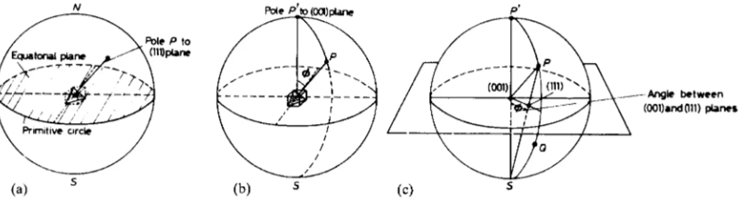
A very small crystal of cubic symmetry is assumed to be located at the centre of a reference sphere, as shown in Figure 2.7a, so that the orientation of a crys-tal plane, such as the (1 1 1) plane marked, may be represented on the surface of the sphere by the point of intersection, or pole, of its normal P. The angle between the two poles (0 0 1) and (1 1 1), shown in Figure 2.7b, can then be measured in degrees along the arc of the great circle between the poles P and P0.
To represent all the planes in a crystal in this three-dimensional way is rather cumbersome; in the stereo-graphic projection, the array of poles which represents the various planes in the crystal is projected from the reference sphere onto the equatorial plane. The pattern of poles projected on the equatorial, or primitive, plane then represents the stereographic projection of the crys-tal. As shown in Figure 2.7c, poles in the northern half of the reference sphere are projected onto the equa-torial plane by joining the pole P to the south pole S, while those in the southern half of the reference sphere, such as Q, are projected in the same way in the direction of the north pole N. Figure 2.8a shows the
stereographic projection of some simple cubic planes, f1 0 0g,f1 1 0gandf1 1 1g, from which it can be seen that those crystallographic planes which have poles in the southern half of the reference sphere are repre-sented by circles in the stereogram, while those which have poles in the northern half are represented by dots. As shown in Figure 2.7b, the angle between two poles on the reference sphere is the number of degrees separating them on the great circle passing through them. The angle between P and P0can be determined
by means of a hemispherical transparent cap graduated and marked with meridian circles and latitude circles, as in geographical work. With a stereographic rep-resentation of poles, the equivalent operation can be performed in the plane of the primitive circle by using a transparent planar net, known as a Wulff net. This net is graduated in intervals of 2°, with meridians in the projection extending from top to bottom and latitude lines from side to side.1Thus, to measure the angular distance between any two poles in the stereogram, the net is rotated about the centre until the two poles lie upon the same meridian, which then corresponds to one of the great circles of the reference sphere. The angle between the two poles is then measured as the difference in latitude along the meridian. Some useful crystallographic rules may be summarized:
1. The Weiss Zone Law: the plane (hkl) is a member of the zone [uvw] if huCkvClwD0. A set of planes which all contain a common direction [uvw] is known as a zone; [uvw] is the zone axis (rather like the spine of an open book relative to the flat leaves). For example, the three planes (1 1 0), (0 1 1) and (1 0 1) form a zone about the [1 1 1] direction (Figure 2.8a). The pole of each plane containing [uvw] must lie at 90°to [uvw]; therefore these three poles all lie in the same plane and upon the same great circle trace. The latter is known as the zone circle or zone trace. A plane trace is to a plane as a zone circle is to a zone. Uniquely, in the cubic
1A less-used alternative to the Wulff net is the polar net, in
which the N–S axis of the reference sphere is perpendicular to the equatorial plane of projection.
Atomic arrangements in materials 17
Figure 2.8 Projections of planes in cubic crystals: (a) standard (0 0 1) stereographic projection and (b) spherical projection.
system alone, zone circles and plane traces with the same indices lie on top of one another.
2. If